Introduction
Iodine. Atomic number 53. Chemical symbol I. Iodine is the rarest of the stable halogens, if we ignore the radioactive elements Astatine (At) and the recently discovered (in 2010) element Tennessine (symbol Ts). Both are extremely rare and extremely unstable.
Iodine is situated in Group 17 of the Periodic Table – for older students like me that is Group VIIA of the table if you are “old school” and were taught the old IUPAC European classification in chemistry classes.
(Just as an aside, the classification of all the elements in the Periodic Table has evolved over time since Mendeleev first devised his periodic system. And at one point there were even differences in nomenclature between the American CAS numbering system and the older European IUPAC system over the years. Thankfully, things now seem to have settled down with a commonly agreed order.)
Iodine is a dark purple, almost black, lustrous crystalline solid at room temperature and pressure and is an element that sublimes when heated, passing directly from the solid phase to the gaseous phase without going through a liquid phase, just like solid carbon dioxide – dry ice. Or so we all originally thought!
In fact, we were all taught in school chemistry classes about the way crystals of iodine sublime when gently heated in a test tube and all chemistry students saw purple vapour liberated from these crystals. However (and this is why I personally find chemistry so interesting as new discoveries are always made when we take a closer look at things), recent examinations of the process actually reveal that solid iodine transitions through a very brief liquid phase before converting to a vapour.
Hmm… time to rewrite the textbooks perhaps!
The electron configuration of iodine is [Kr]4d105s25p5. The seven electrons in the 5s and 5p orbitals in shell number 5 are the valence electrons that take part in chemical reactions. Like the other lighter halogens fluorine, chlorine and bromine, iodine is one electron short of achieving a full octet, the most stable energy configuration. As such, iodine, in common with the other halogens, reacts readily with many chemical reagents to complete its outer shell of 8. Consequently, elemental iodine by itself is unstable and combines rapidly with a second iodine atom in order to share a pair of electrons and complete a stable 8-electron octet. The most stable state of iodine is therefore the diatomic molecule I2.
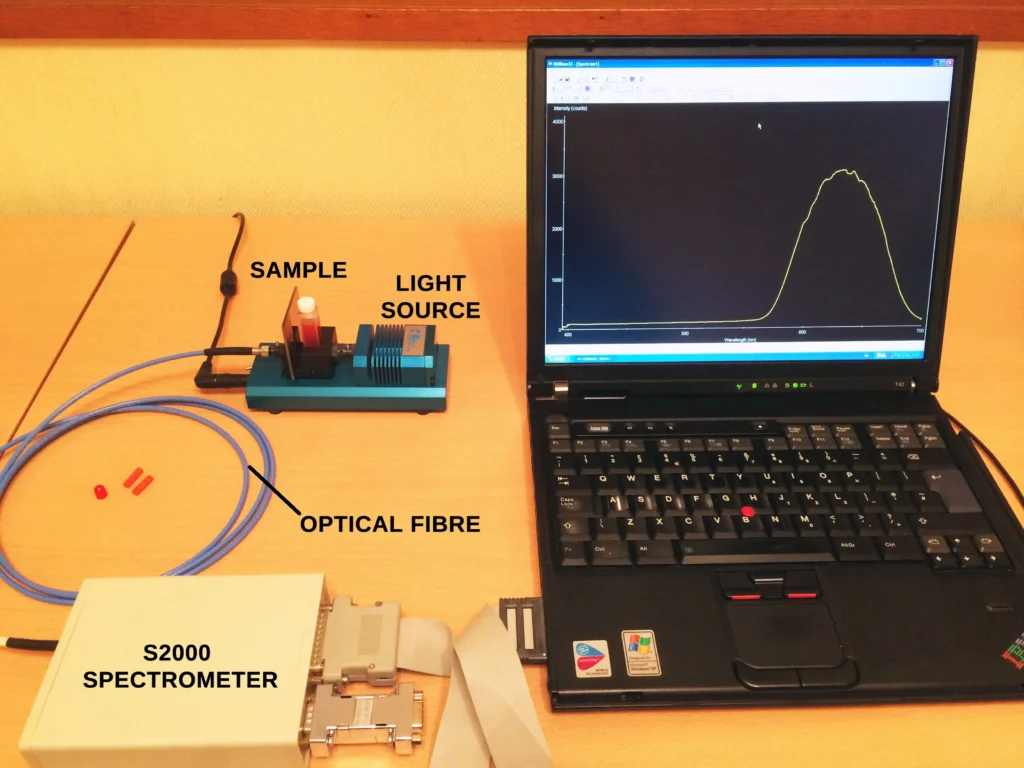
In line with the main subject matter of this post, we are here to have a look at the absorption spectrum of iodine and the best way to do this is to examine iodine in the gas phase by firing a beam of light through it.
But first, we have to consider a little theory in order to understand what is going on. This will represent Part 1 of this 2-part post.
Basic Theory - Energy Levels of a Diatomic Molecule
The total energy Etotal of a diatomic molecule can be described, to a good approximation, by the sum of the individual energies that describe its possible types of motion:
Etotal = Etrans + Erot + Evib + Eelec.
Etrans is the energy associated with simple displacement (translation) of the molecule through three-dimensional space,
Erot is the energy associated with rotation of the molecule around its centre of mass,
Evib is the energy associated with vibration of the molecule,
and Eelec is the energy associated the electrons in the different atomic and molecular orbitals (ground state, excited state, etc.).
This is the basis of the Born-Oppenheimer approximation, a well known mathematical approximation frequently applied to the dynamics of rotating and vibrating molecules. The assumption is that the wave functions of the atomic nuclei and the electrons in a molecule can be treated separately. It is based on the fact that the nuclei are much heavier and slower than the fast moving and lighter electrons. It greatly simplifies quantum mechanical calculations in chemistry and is widely used. It was first proposed by Max Born and J. Robert Oppenheimer in 1927 during the rapid development quantum theory.
For all practical purposes, the translational energy component in the above expression can be neglected. Although translational energies are formally quantized in space, any quantum effects are so small as to be negligible when compared to the energies associated with rotation, vibration and electronic changes. Therefore translational energy changes are not considered further.
A typical energy level diagram for a diatomic molecule can be described simplistically and schematically using the following diagram for two different electronic energy levels (shown not to scale):
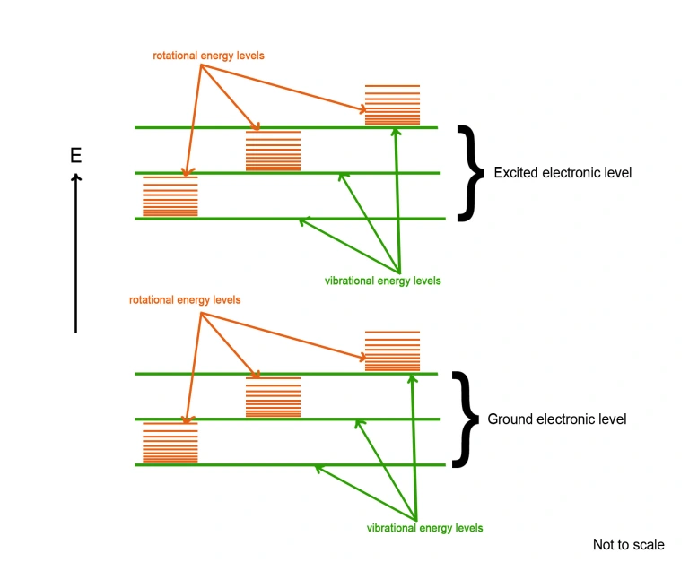
Within each electronic state there is a “ladder” of vibrational energy levels of increasing energy (shown in green in the above diagram). Similarly, within each vibrational energy level, there is a series of rotational energy levels of increasing energy (shown in orange).
It is clear from the above diagram that the energy required for an electron to transition from one rotational energy level to a higher rotational level is quite small, and very much less than the energy required for the electron to transition from one vibrational energy level to another.
Differences in energy between two consecutive rotational levels is of the order of 1 cm-1. An energy gap of this size falls within the microwave region of the electromagnetic spectrum. Thus, pure rotational spectra within the same vibrational energy state are most often observed by microwave absorption techniques.
[The unit cm-1 (reciprocal centimetre) is commonly used in spectroscopy, especially in the UV, visible and IR. It is called the wavenumber with the symbol ῡ. One wavenumber is defined as the number of wavelengths per centimetre and so
where lambda, λ, is the wavelength expressed in cm and ω = 2πυ is the angular frequency. As an example, a visible wavelength of 400 nm in wavelength is equivalent to 25,000 in wavenumbers (cm-1) ]
When we consider vibrational levels, energy differences between adjacent states are of the order of 1000 cm-1 and energy changes of this magnitude fall within the infrared (IR) region of the spectrum. IR spectrometers and spectrophotometers are employed to study the vibrational properties of molecules by exciting them with IR (thermal) radiation.
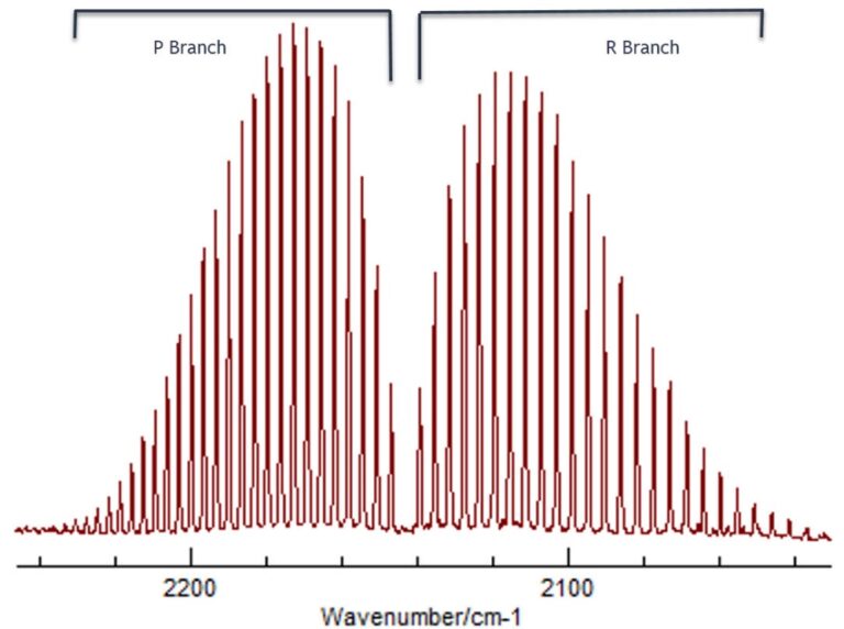
What should also be stated is that besides exciting vibrational states, rotational energy transitions will always take place simultaneously between different rotational energy levels. This gives rise to what is called rotational fine structure in any vibrational spectrum. A good example is the molecule carbon monoxide (CO) where what are called the P branch and R branch envelopes correspond to vibrational energy levels and the fine structure under each branch represents the various rotational energy transitions. More details about rotational and vibrational fine structure of diatomic molecules can be found at this link.
In a similar way, differences in energy between electronic energy levels are very much larger, and range from around 10,000 cm-1 up to 100,000 cm-1. Energy changes of this magnitude extend from the UV region and all through the visible and these transitions involve exciting an electron from its lowest electronic energy (ground) state to the next highest electronic energy (excited) state.
So, to summarize:
Pure rotational level transitions involve energy changes of ~ 1 cm-1 and occur in the microwave region,
Vibrational level transitions involve energy changes of ~ 1000 cm-1 and occur in the IR region,
Electronic energy level transitions involve energy changes of ~ 20,000 to 100,000 cm-1 and occur in the UV and visible regions.
The Vibrating Diatomic Molecule
Simple Harmonic Motion
We can consider a diatomic molecule as a pair of billiard balls (atoms) connected via a metal spring (the chemical bond). This is the popular ball and spring model of the molecule and this treatment describes the molecule undergoing simple harmonic motion. As such the molecule is referred to as a harmonic oscillator. It is reasonably accurate up to a point. The vibration of this molecule undergoes simple harmonic motion, as can be seen in this simple animation (courtesy of the Specac corporation) as the bond between the two atoms is alternately compressed and stretched.
The vertical axis E (which is sometimes called V when dealing with vibrational energies and spectra) is the potential energy and r is the internuclear distance (the bond length) along the horizontal axis. As the spring (bond) is compressed, a repulsive electrostatic force builds up and rapidly increases as the two atoms come together. A point is reached where the repulsive force dominates and pushes the atoms away. As the atoms move apart a force of attraction starts to build again to pull the atoms back together again. The end result is that a state of equilibrium exists at a point of lowest stored energy in the molecule at an internuclear distance re, known as the equilibrium bond distance.
Assuming the vibration only involves small displacements of the bond length, r, from the equilibrium bond distance, re , the restoring force f necessary to change the direction of the atoms to maintain vibrational motion is proportional to the displacement (x) of the bond length from its equilibrium value, re. Thus x = r – re , and the proportionality expression is given by
(1) f = – k x
This equation is known as Hooke’s Law and applies to molecules as well as everyday objects undergoing small displacements and exhibiting simple harmonic motion. Such objects are referred to as harmonic oscillators. The variable k is called the force constant; its value is relatively small for weakly bonded atoms and increases with increasing bond strength. Thus a triple bond will have a larger force constant than a double bond, which in turn will have a larger force constant relative to a single bond. It is measured in units of Newtons per metre (N m-1).
The potential energy (which we will now call V(x) instead of E used in the above animation) is a function of the displacement x and is equal to
(2) V(x) ≅ ½kx²
However, we all know that molecules do not behave as classical particles. The laws of quantum mechanics determine the vibrational energy of any molecule and only a limited number of discrete energy levels is allowed. The values of these discrete energy states are obtained from solutions of the Schrodinger equation for a vibrating molecule. The energy states are therefore quantized in terms of the vibrational quantum number υ and the resulting allowed energies of vibrational levels, Eυ are given by
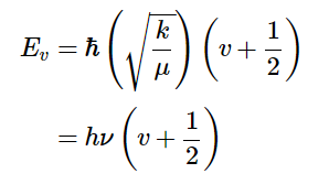
where μ is the reduced mass and ħ is Planck’s Constant divided by 2π. [Note that the frequency, ν, and the vibrational quantum number υ are different symbols.]
From the above expression we obtain the vibrational frequency:
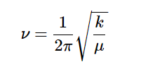
The reduced mass μ = m1m2/(m1 + m2) in units of a.m.u. (atomic mass units). For example, for the iodine molecule, μ = 1.05 x 10⁻²⁵ kg.
Equation (3) implies that the quantized vibrational energy levels are equally spaced for a harmonic oscillator and equal to hv. In vibrational spectroscopy the wavenumber is usually used (as explained earlier) and it is conventional to express the vibrational spacing hv as hcῡ , where ῡ is the vibrational wavenumber and c is the speed of light.
With this convention the vibrational energies are then referred to as “Term Values” and are labelled G (v). Equation (3) is therefore often expressed as
(5) G(v) = ῡ(v + ½)
Anharmonicity
For large displacements of the atoms in a vibrating diatomic molecule, Hooke’s Law is no longer obeyed. The molecule no longer undergoes simple harmonic motion but instead behaves as an anharmonic oscillator. As a consequence, a more accurate representation of the potential energy curve is shown in this animation (courtesy of Darekk2 and Wikipedia Creative Commons), in this case for atoms of different mass.
With this more accurate representation (which is still a model), as the bond is compressed at shorter bond lengths the potential energy increases steeply for very little change in internuclear distance. At longer bond lengths the bond starts to weaken and the force constant decreases. If the bond is stretched even further it finally breaks and the molecule dissociates into two neutral atoms.
The vibrational energy levels of this potential energy curve are not equally spaced and the vibrational motion is not harmonic (it is anharmonic). As shown in the animation they become closer together and converge at the bond dissociation limit.
We can express this behaviour mathematically by adding successively smaller terms to equation (5) above to give:
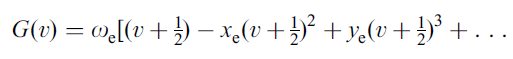
where xe,, ye,… are called the anharmonicity constants and ωe is the vibrational frequency (the “harmonic” frequency of the oscillator).
During the early development of quantum mechanics and spectroscopy in the 1920’s and 1930’s there were several attempts to modify the general expression for equation 2. The aim was to adapt the harmonic oscillator model in order to take into account anharmonic behaviour of molecules that would better agree with actual observations. The most successful modification, and the one often used, is the Morse potential function, named after American physicist Philip M. Morse who proposed it in 1929. The Morse function is:
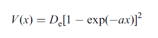
where x is equal to r – re and a is a constant. The Morse potential energy function is still only an approximation, but it has the great advantage that V(x) → De, the bond dissociation energy, as x → ∞, when the bond finally breaks.
A schematic of the Morse potential curve compared to the simple harmonic oscillator, can be seen here:
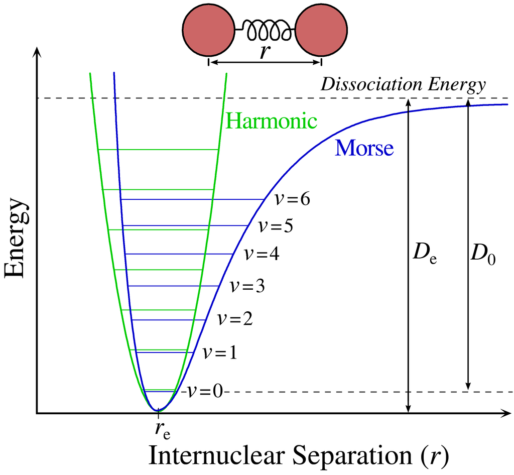
The green curve, which is a parabola, is the simple harmonic motion for the molecule explained in the first animation earlier. The blue curve is the more accurate Morse potential curve that describes the variation in potential energy of a diatomic molecule as a function of internuclear distance.
The ν = 0, ν =1, ν = 2, … are the quantized vibrational energy levels as explained previously and ν is called the vibrational quantum number. The bond distance is r and re is the equilibrium internuclear distance. De is the bond dissociation energy measured from an absolute zero point on the x axis and D0 is the actual energy needed to break the bond, as measured from the lowest vibrational energy level ν = 0.
As potential energy increases, the vibrational levels become closer and closer together until the bond finally breaks and neutral atoms fly apart. The blue curve depicts the distance between the nuclei of each atom increasing to infinity at the bond dissociation limit.
By examining the vibrational structure in the spectrum of a diatomic molecule, we are able to calculate some important parameters for the molecule such as its bond dissociation energy D0. A useful way to obtain a value for D0 is to record experimentally as many transitions in the vibrational spectrum of the molecule as possible.
In practice, D0 can therefore be measured by summing all the small vibrational energy differences for all the vibrational energy states. Expressed mathematically,
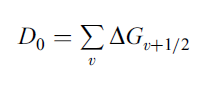
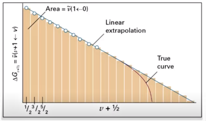
In short, D0 is the sum of all vibrational energy separations. If we neglect (truncate) the higher order terms in equation (6), with the exception of the squared term, then ΔGv+1/2 becomes a linear function of v. We can then construct a graph of ΔGv+1/2 versus (v + ½), and the bond dissociation energy D0 will be equal to the area under the graph.
A least squares fit (regression line) is usually calculated and linear extrapolation of the line to ΔG = 0 is performed in order to determine the area and obtain D0.
This approach is known as the Birge-Sponer Method, named after Raymond T. Birge and Hertha Sponer, the two physical chemists who developed the technique in 1926.
In practice, the Birge-Sponer method does have some limitations. Both authors were, of course, well aware of these limitations when they first proposed the approach.
For many diatomic molecules, for instance, only a limited number of vibrational transitions may be measurable by experiment. In some cases the appearance of vibrational transitions can disappear well before the dissociation limit is reached because these very high vibrational states are only sparsely populated or totally unpopulated. As a result the graph often must be extrapolated to the point where ΔGv+1/2 = 0. Moreover, the plot will be a straight line only if the higher order anharmonicity constants are neglected.
Nevertheless, the Birge-Sponer method has proven to be very useful over the years for an estimation of the bond dissociation energies of diatomic molecules and it provides a useful upper limit to the value of D0.
The technique arrived at a time in the last century when the main experimental goal of physicists and chemists working in the field of spectroscopy was to obtain the best possible measurements for these fundamental parameters of simple diatomic molecules.
With this basic theory in hand, we can now move on to the experimental stage. We will prepare a sample of iodine and record its absorption spectrum in a simple home experiment.
This is described in Part II of this post.