Introduction
In this post the emission spectra of the Noble Gases are presented.
The noble gases constitute the last group (Group 18) in the Periodic Table of the elements. Emission lines obtained from the spectra of these noble gases can be very useful for the calibration of a spectrometer.
Historically, these elements were called the Inert Gases, because it was thought that nothing appeared to react with them chemically. This, however, is not exactly true. Some of these elements do in fact react, under very special conditions, with other elements such as the highly reactive halogens.
Good examples of this are with pulsed UV laser light sources known as excimer or exciplex lasers. These deep UV lasers generate excited dimers (excimers) and complexes (exiplexes) under the right conditions. XeCl* and KrF* are good examples, where the * denotes an excited state. These excited complexes are produced in the gas phase by reactions between xenon and chlorine, and by krypton and fluorine, under carefully controlled energy and pressure conditions.
So at least some of the noble gas elements can no longer be described as being strictly inert.
In order of increasing atomic number, the naturally occurring noble gases are helium (He), neon (Ne), argon (Ar), krypton (Kr), xenon (Xe) and the radioactive element radon (Rn).
There is also a highly unstable and radioactive element given the official IUPAC name Organesson. It was first synthesized in a nuclear reactor in 2002, by a team of American and Russian nuclear physicists, and has an atomic number of 118. Organesson has the distinction of having the highest atomic and mass number of all known elements. Since only a few atoms have ever been detected in the laboratory, it will be mentioned no further here!
Since many of these blog posts concern spectroscopy, the main goal for this one is to present the emission spectra of the non-radioactive Noble Gases. They can easily be produced in a home lab by any amateur scientist with the right basic equipment.
But before we get to the actual experiments, we need to say a few words on spectral lines.
Spectral Lines, Line Widths and Line Broadening
First of all, why are they called lines?
The term spectral line dates back to the early days of observing and recording visible spectra with bench top spectroscopes and through telescopes with a spectroscope attached. The line is simply an image of the slit of the spectroscope.
An old image of such a spectrum is shown here. These spectra were usually recorded on a photographic plate or film, then the plate developed:

The above spectrum of the CH radical was recorded on a photographic plate by A. E. Douglas and G. Herzberg, and published in the Astrophysical Journal in 1942. It was re-presented in Gerhard Herzberg’s Nobel lecture in 1971 after he received the prize.
Modern spectrometers today use highly sensitive solid state linear and array detectors, often CCD’s or CMOS sensors, in the visible region of the electromagnetic spectrum. Dispersed light from the spectrometer is then generated automatically by software to produce a plot, with signal intensity (counts) on the y-axis and wavelength on the horizontal x-axis.
An example is the spectrum below of a krypton gas pencil-type discharge lamp that I recorded 20 years ago now. (Note that wavelength axis is in Angstrom units (Å) and not nm):

The lines, whether they are dark lines on photographic film or peaks on a plot, are simply images of the entrance slit of the spectroscope across the different wavelengths. Spectrometer entrance slits are typically a few millimetres long and vary in width from 10 microns to several hundred microns.
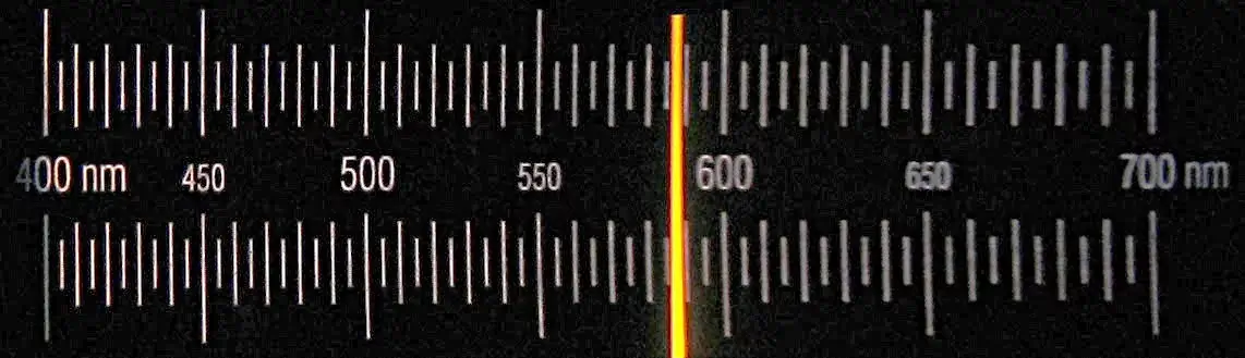
If the lines are seen in emission, such as from a sodium lamp or a flame, the line spectrum would be a bright narrow yellow line. The sodium line at 589 nm, on a dark background (left image below) is an example. If the lines are seen in absorption, such as the well known Fraunhofer lines seen in the Sun, the spectrum becomes a series of dark lines on a bright background spread throughout the visible spectrum (right image):

It is important to mention that no spectral line corresponds to an infinitely narrow energy transition. This is because there are a number of fundamental theoretical, and also practical, limitations that determine the absolute width of a spectral line that can be observed.
The processes that govern the widths of spectra lines are briefly described below.
Natural Broadening
The most fundamental of these limitations is natural broadening. It is sometimes referred to as lifetime broadening, since it is intimately related to the lifetime (i.e. the “residence” time) of a particle, such as an electron, in an excited state, before it loses energy by returning to a lower energy level.
This means that there is a fundamental restriction on the width of a spectral line. It has its origins in quantum mechanics and the Heisenberg Uncertainty Principle, placing a natural limit to the width of any line and transition.
Briefly, the Uncertainty Principle determines a limit on a pair of measurement variables for an atomic system, such as momentum and position, or energy and time, in the following way.
Heisenberg’s original paper, in 1927, dealt with the changes in momentum and position of a particle and derived his famous approximation
Δp x Δq ≈ h,
where p is momentum, q is position of the particle at any instant and h is Planck’s Constant.
The expression was elaborated further by Hermann Weyl and Earle Kennard a few months later in late 1927 and early 1928, during those revolutionary years in quantum physics. This refinement described these uncertainties in terms of standard deviations (sigma quantities, σ).
This led to the now famous expression
σx x σp ≥ ħ/2π,
where ħ is called the reduced Planck Constant and is equal to h/2π.
The Uncertainty Principle can be expressed in its “energy-time” equivalent version by the equation:
ΔE x Δt ≈ h/2π.
In this version, which is intuitively more understandable when it comes to spectroscopy and energy transitions, means that the product of the uncertainties, in the energy and time domains, cannot be less than a certain value, namely h/2π.
Since the lifetimes of atoms (and also molecules) in excited energy states typically range from nanoseconds to microseconds, then Δt, the time factor in the above expression, will exhibit this same intrinsic time uncertainty.
Now the Planck Equation is defined as ΔE = hν, where v is the frequency of the radiation the transition. Any uncertainty in the value of frequency, Δv, will therefore be
Δv = ΔE / h.
If we plug this equation into the Uncertainty Principle expression, we end up with
Δv = 1 / 2πΔt.
This is the intrinsic (natural) uncertainty in the frequency (or wavelength) of an emitted or absorbed photon of light. It represents the fundamental limit on the line width. The value is extremely small, in reality on the order of 0.00001 nm. This is certainly well below the resolving limit of even the highest resolution spectrometers. It is generally considered negligible in any practical spectroscopic measurement and as such can be safely ignored.
Doppler Broadening
Doppler broadening (also called thermal broadening), as the name implies, arises from the Doppler Effect.
As a reminder. the Doppler Effect explains why the siren from an ambulance travelling towards an observer appears to have a frequency (or pitch) apparently higher than it really is, and lower when it is travelling away from the observer.
In any sample of gas at a certain temperature, some photons that are emitted will be moving away from the observer (red-shifted and of longer wavelength) and some emitted will be moving towards the observer (blue-shifted and of shorter wavelength).
The resulting spectral line, therefore, is a combination of all these different directional possibilities, and this consequently broadens the spectral line that is produced. Moreover, these Doppler shifts depend on the temperature of the gas. The higher the temperature, the broader the line that is produced because the distribution of velocities of particles in the gas is broader and wider.
The Doppler broadening effect is described mathematically by a Gaussian line profile, as explained in more detail here.
Pressure (Collisional) Broadening
When collisions occur between atoms or molecules in the gas phase there is an exchange of energy. This effectively leads to a broadening of the energy levels. If τ is the mean time between collisions, and each collision results in a transition between two states, there is a line broadening Δν of the transition, where
Δν = (2πτ)-1
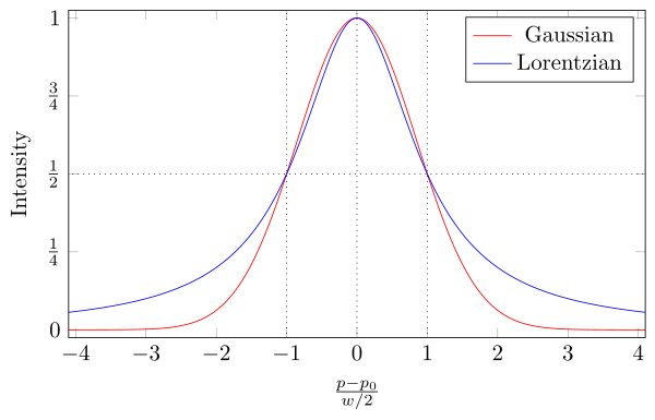
This is derived from the uncertainty principle in a similar way as explained above. This is called pressure broadening and, like natural line broadening, it is homogeneous. It becomes predominant and important in high density gas emission spectra (which are essentially plasma emissions). It usually produces a Lorentzian spectral line shape that has a sharper peak and longer wings relative to a Gaussian line profile, as shown here:
Saturation (Power) Broadening
When in equilibrium, the populations of energy levels are given by the Boltzmann distribution law. These populations are maintained through energy exchanges by collisions between the particles (atoms, molecules, etc.)
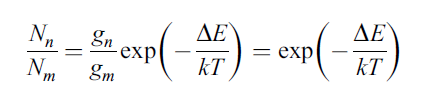
Nn and Nm are respectively the number of atoms (or electrons, etc.) in the higher energy state n and the lower energy state m, ΔE is the energy difference between the two states, k is Boltzmann’s constant and T the temperature in degrees Kelvin. gn and gm are the degrees of degeneracy of the states n and m.
When the ground and excited energy levels, m and n, are close together, the population ratio Nn/Nm is close to 1 at equilibrium. A consequence of this is that the equilibrium can be seriously disturbed when a sample is subjected to increased radiation power, as can happen with some absorption experiments. The Beer-Lambert law then breaks down and the molar extinction coefficient, ε, becomes dependent on the light intensity, I.
At this point, saturation is said to occur and line profiles become broadened as a result. The closer the energy levels n and m are, the more easily this can occur. It is therefore be quite common with microwave and millimetre wave spectroscopy, which deal with the very small energy changes between rotational levels in molecules. Nevertheless, saturation broadening can still take place in visible and UV spectroscopy, such as with high power lasers.
One effect of saturation is to decrease the maximum absorption intensity of a spectral line. The central part of the line becomes flattened and the intensity of the wings is increased. The result is that the line is broadened, and the effect is known as power, or saturation, broadening.
An example of this effect in the visible is a spectrum that I obtained (over 20 years ago now!) from a high pressure sodium street light (HPS lamp) down the road from where I lived at the time. This spectrum was obtained with a small hand-held spectrometer (an Ocean Optics S2000 spectrometer) attached to a Meade 11-inch Schmidt-Cassegrain telescope (SCT) aimed at the lamp.

The sodium emission line in the above spectrum at 589 nm is very significantly broadened with a strong dip at the peak maximum due to self-absorption. Basically, any photons emitted on the centre line are immediately re-absorbed by neighbouring atoms under these high pressure and intensity conditions. The end result is that there is a strong dip in the emitted intensity at the peak maximum.
Remarkably, I discovered this old spectrum of mine online, after 20 years! It formed part of a review of some commercial spectrometers that I wrote at that time.
The interested reader can find this review at http://users.erols.com/njastro/faas/pages/paper001.htm
The review formed the basis for a chapter in the book Practical Amateur Spectroscopy, available here:
The Spectra
At last, we come to the actual spectra.
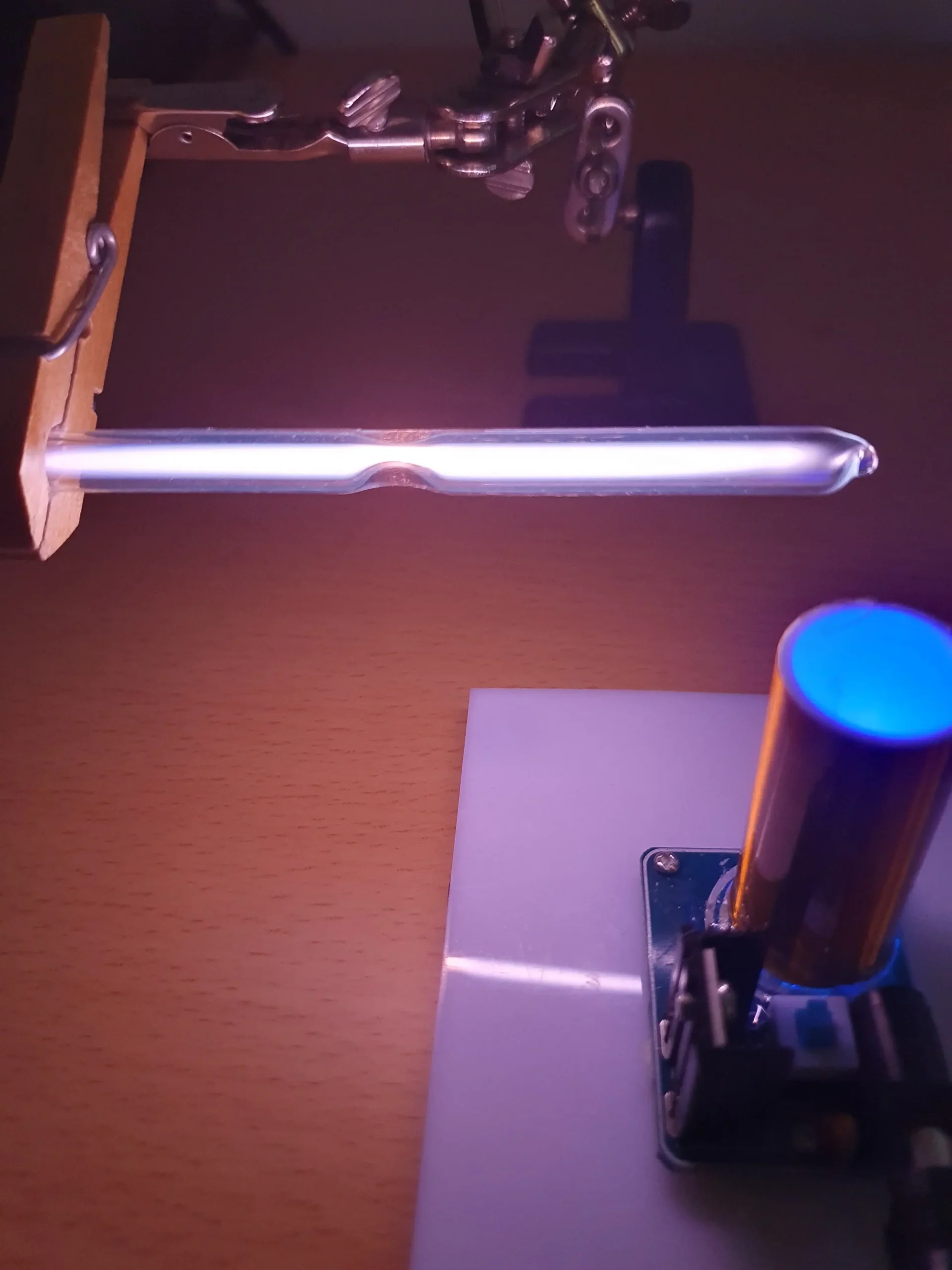
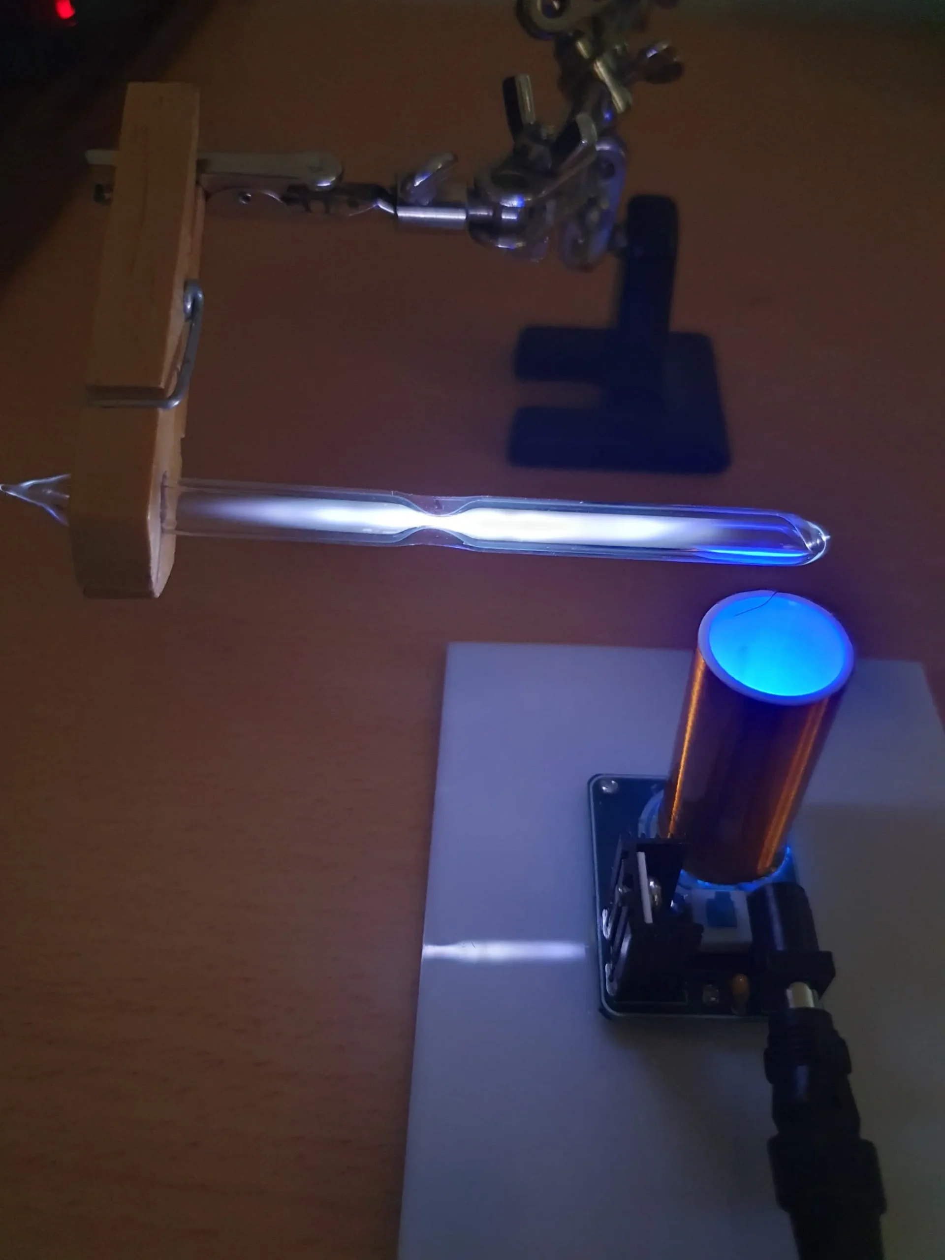
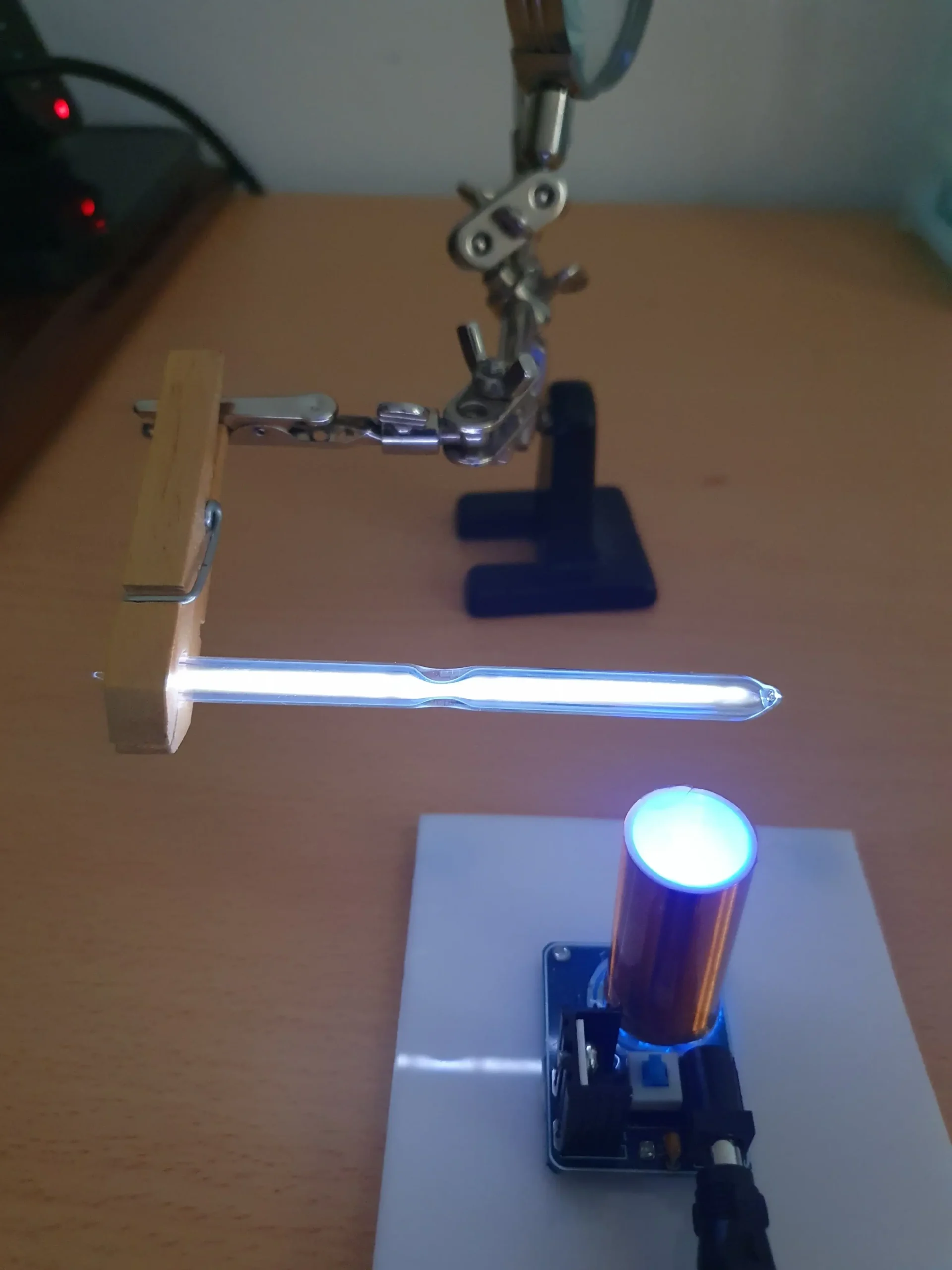
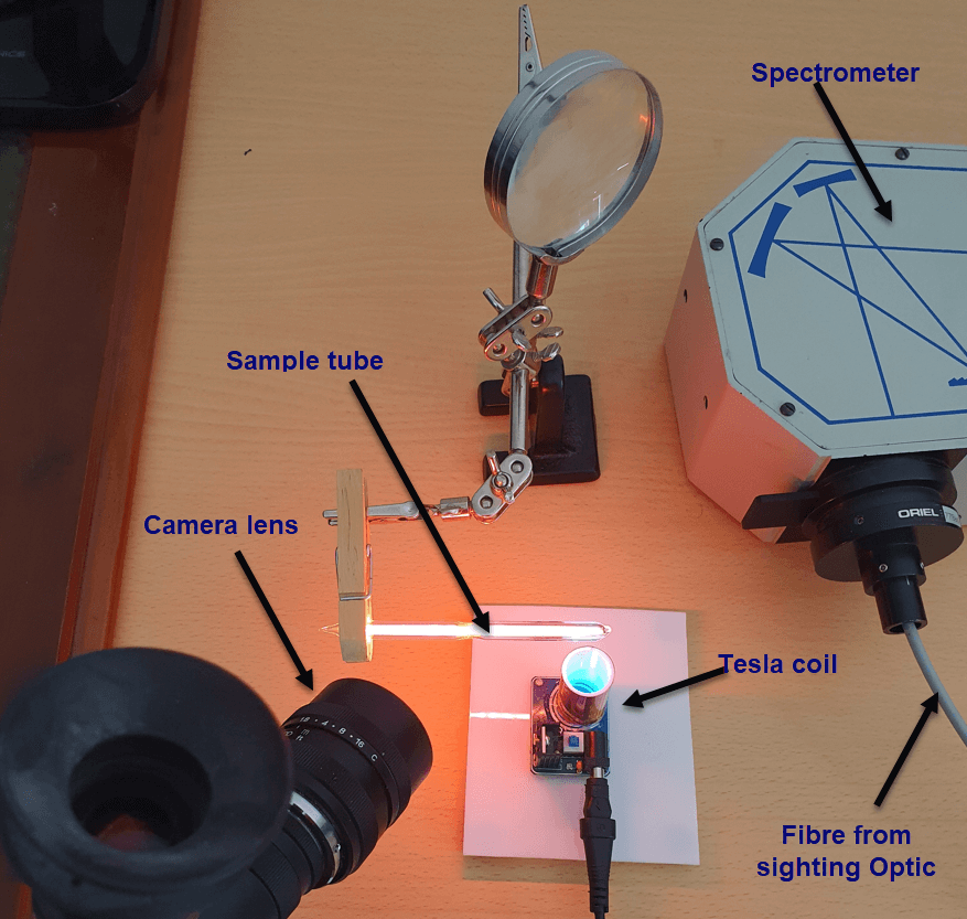
A small Tesla coil is a very handy tool to induce and generate high frequency alternating current discharges. The coil generates a very high voltage (several 10,000V or more) but at extremely low current and extremely high oscillating frequency. Under these conditions, the Tesla coil is perfectly safe.
Mini-Tesla coils are widely available online and cost only a few dollars.
Noble gas discharge tubes were purchased from Smart Elements in Austria, a useful source for items of this kind.
This short video demonstrates how the coil produces the discharge, in this case with a glass sample tube containing neon at low pressure:
And the basic experimental setup can be seen below. The camera lens and spot measuring device (sighting optic) are described in detail elsewhere.
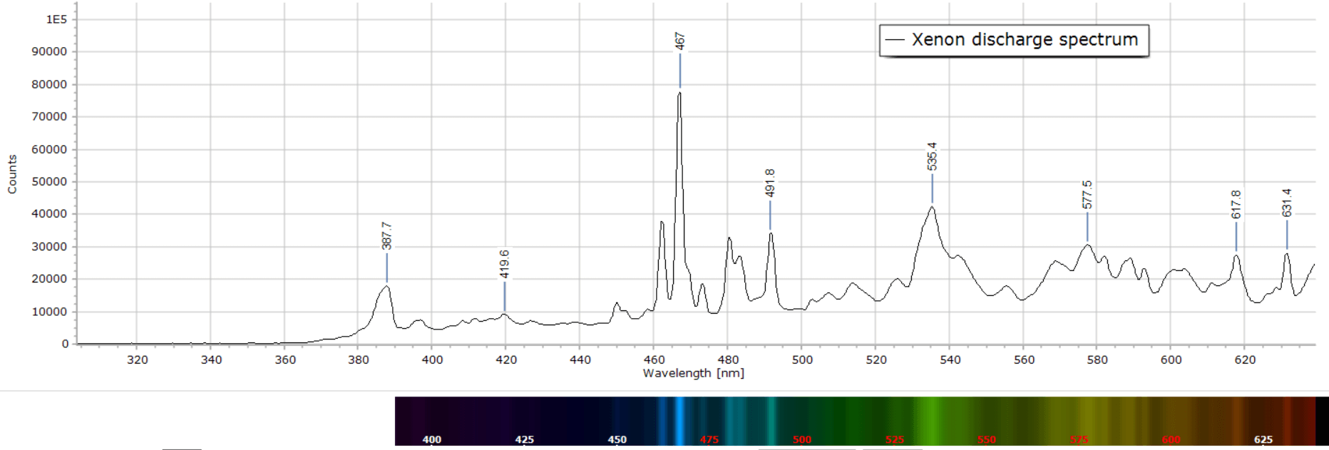
Images of the different atomic discharges and resulting emission spectra are presented in the following gallery:
The wavelength accuracy of the lines in these spectra is +/- 1 nm. They can be useful to the home experimenter for the calibration of a spectrometer, whether home built or purchased.