Factors Affecting Spectrometer Performance

7 Minute Read
Factors affecting line profile

Introduction

There are a number of technical constraints to consider when selecting a spectrometer for a particular application, whether this involves purchasing a commercial model from the wide range of relatviely low cost mini-spectrometers available these days, or whether one is designing and home-building a spectrometer from scratch.

In this post we shall consider some of the principle choices and compromises that need to be evaluated without going too deeply into the technical details.  A much more technical and theoretical discussion will be posted in the near future.

Focal Length

The first constraint to examine is the focal length. When it comes to compact mini-spectrometers that use optical fibres, it is fair to say that the pioneer in this field was the company Ocean Optics Inc. (now rebranded as Ocean Insight) who began to commercialize these small devices in the mid 1990’s from their home in Dunedin, Florida. Since that time the competition has caught up and today, a number of manufacturers sell very similar products. Companies such as Avantes, Stellarnet, Thunder Optics, Edmund Optics, Thorlabs and several others, in addition to the inevitable Chinese copies, all sell small, virtually hand-held spectrometers for field operations, as well as for the lab.

A common feature of many of these devices is their small physical size (not much larger than the palm of your hand!) and their inter-connectability with sample holders, light sources and a PC via optical fibres and a USB cable. An equally similar feature is the generally small focal length of these devices, typically from around 50 mm to 100 mm at most.

However, there are no two ways about it. If you need a spectrometer with the advantage of small physical size for portability, perhaps field operations, and one that is also lightweight, then this will restrict and determine the final focal length of the optical platform. If the focal length is limited, the overall spectral resolving power of the instrument will be similarly limited. Fortunately today, these drawbacks can be offset, to some extent, by the use highly sensitive detectors that are integrated into these small devices that allows them to obtain practically useful results.

Avantes Optical Bench
Fig.1 Internal design of an Avantes spectrometer optical bench
Stellarnet Blue Wave
Fig.2 Stellarnet BlueWave spectrometer

Fixed or Interchangeable Gratings?

Until recently all small hand-held spectrometers use fixed gratings and therefore the amount of spectral dispersion is pre-configured when manufactured. If we increase the focal length of the spectrometer slightly, say to 125mm and higher, the device becomes slightly physically larger, obviously heavier, and the possibility of having different diffraction gratings becomes available in the design.

Having interchangeable gratings means that different wavelength ranges can be selected and focused on the detector. This is the case with the MS125 spectrograph described in detail in this post. For larger focal lengths still, say ¼ metre focal length and higher, multiple gratings that have different dispersions (number of grooves per mm) and blaze angles become possible. These are often attached to a rotatable turret and computer controlled. But these advantages can really only be incorporated using a much larger optical bench. With these larger spectrometers, grating changes are often automatic and are software controlled.

Detectors

For recording spectra in the visible region, standard CCD or CMOS sensors are almost always used. For applications in the infrared region InGaAs (Indium Gallium Arsenide) sensors are employed which extend the detection capability up to around 2.2 to 2.5 μm.

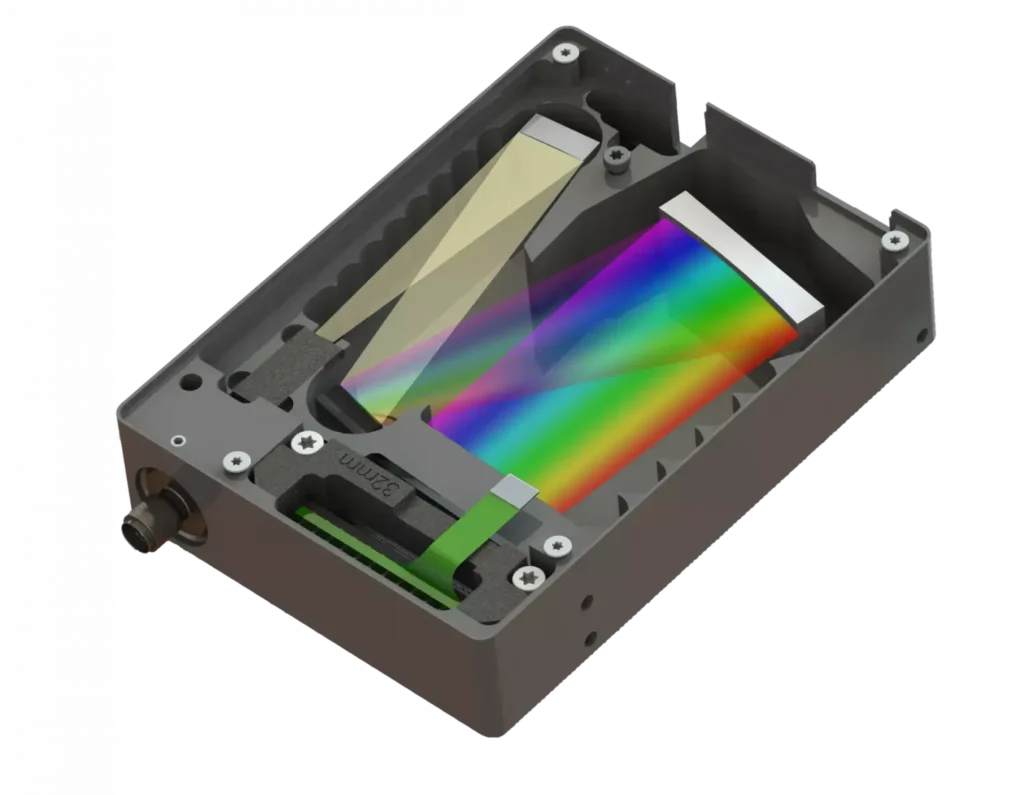
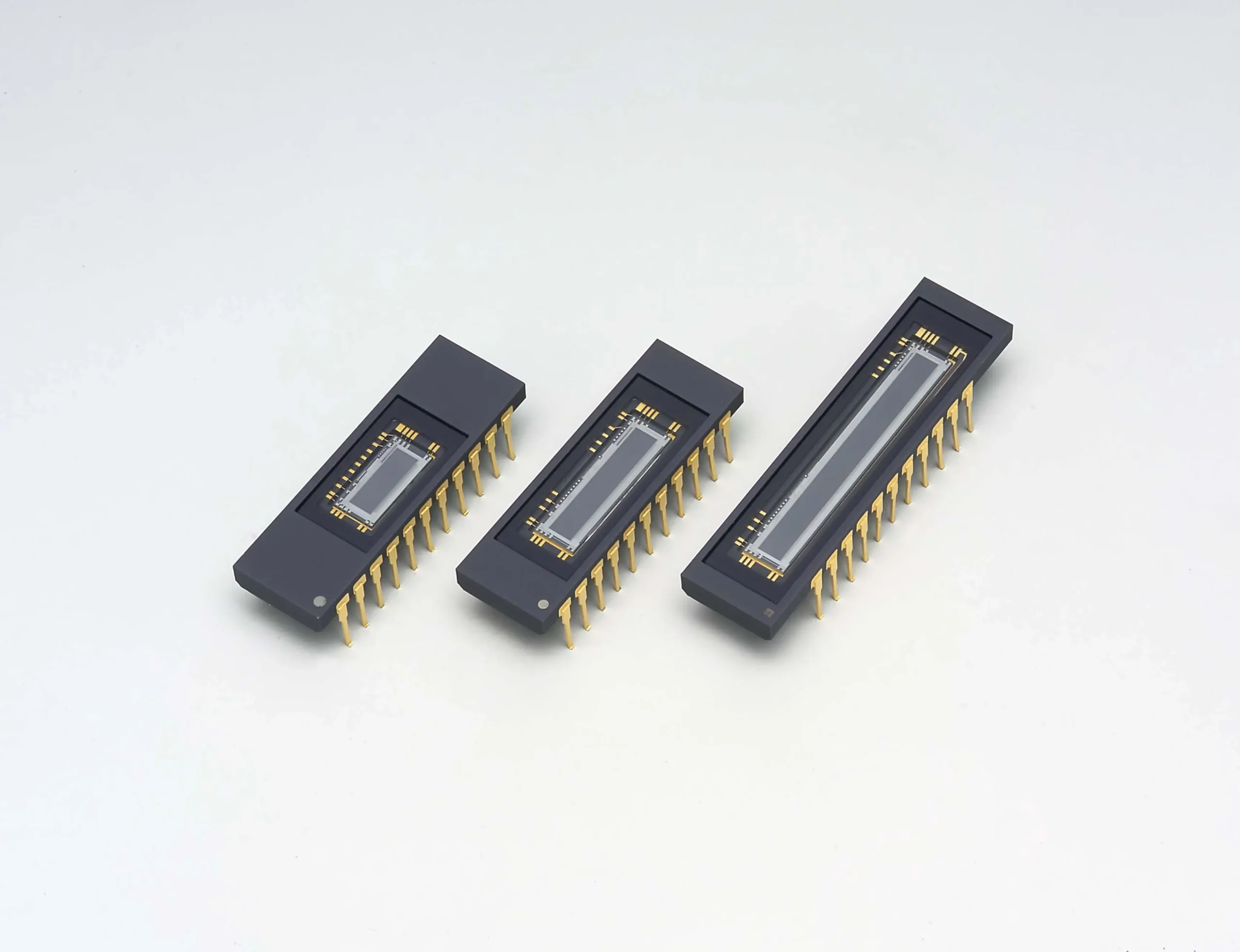
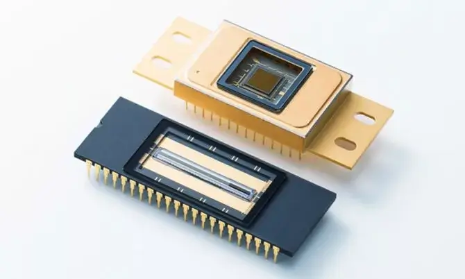
   For conventional spectroscopy (as opposed to imaging applications) all these light sensors are “linear” in design and consist of a finite number of pixels corresponding to the individual electrode structures fabricated on the silicon wafer. The dispersed light from the grating is designed to fill these linear sensors in the horizontal direction of dispersion as much as possible.

   The earliest generation of sensors had only 512 pixel elements. Soon after, sensors with 1024 pixels became available. Then came sensors with 2048 pixels and today sensors with 4096 pixels have recently been introduced. So we have seen a steady and progressive increase in the number of individual light sensitive elements packed into a light sensor chip, as wafer fabrication methods and designs have steadily improved.

   These improvements parallel, in an entirely analogous way, the developments in microprocessor chip manufacturing technology using deep UV and X-ray microlithography on silicon wafers. These techniques have consistently reduced transistor feature size for the last 40 years or so to achieve improved CPU performance.

(As an aside, this relationship is known as Moore’s Law, named after Gordon Moore, the co-founder of Fairchild Semiconductor and a former CEO of Intel, who posited the relationship in 1965.)

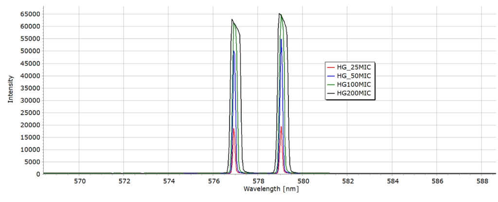
For light sensors, these improvements have led to an increase in the spectral resolving power of the spectrometer (all other things being equal).

The actual dimensions of the light sensitive area in these sensors is typically about 25 mm in length and 1–3 mm in width, although sensors with both spectroscopic and imaging capability can, and do, have larger dimensions in the non-dispersion direction. If the primary application is for spectroscopy, a pixel count of 128 or 256 in the non-dispersion direction is perfectly adequate and can still exhibit some limited imaging capability for examining, for example, extended light sources.

Hamamatsu linear sensors
Fig.3 Linear CMOS sensors from Hamamatsu
Fig.4 Infrared sensitive InGaAs sensors

Entrance Slit Width

The width of the entrance slit to a spectrometer is also a very important parameter that plays an important role in optimizing efficiency for a given application. It is also referred to as spectral throughput, “light grasp” or  Etendue (from the French for how spread out the light is that enters the slit).

The mini fibre-optic spectrometers mentioned earlier usually (but not always) have fixed slits that are optimized with the instrument for a given wavelength region. They offer the best achievable compromise between light throughput (étendue) and spectral resolution.

Larger focal length instruments almost always will come with interchangeable slits of fixed width or even a variable slit that can be adjusted by a micrometer screw or dial (Figures 5 and 6).

50 and 100 micron slits
Fig.5 Two fixed slits from an Oriel-Newport MS125 1/8m spectrograph
Variable Slit
Fig.6 Variable aperture slit from a Jobin Yvon spectrograph. The dial on the top sets the slit width and the side slider can adjust the slit height.

Effect of Slit Width on Line Profile

A clear example of the effect that changing the slit width can have on the spectral line shape (or profile) can be seen in Figure 7. These are two well known emission lines produced by a Mercury or Mercury-Argon calibration lamp at 576.96 nm and 579.07 nm (5769.6Å and 5790.7Å).

An increase in slit width from 25 μm through to 200 μm results in a progressive degree of line shape broadening and at 200μm the line shape exhibits significant distortion of what should be, in principle, (since this is a single atomic emission line) a symmetrical profile. This distortion at very high slit widths is usually due to scattered light but other factors, such as poor f/number matching can be the cause. 

Factors affecting line profile
Fig.7 Effect of increasing entrance slit width on spectral line shape.

A final example of slit width effects is provided in Figures 8, 9 and 10 below for the sodium D lines in the solar spectrum at around 589 nm. With a slit of 25 μm the sodium doublet is very well resolved and close to the theoretical separation (Fig. 8). At 50μm the two lines can still be resolved and identified but have started to broaden significantly (Fig. 9). Finally at 200μm, line broadening has become so strong that the overall profile is a convolution of the two overlapping absorption lines in the Sun’s spectrum.

With a 25 micron slit
Fig.8 A 25 micron slit
With a 50 micron slit
Fig.9 A 50 micron slit
With a 200 micron slit
Fig.10 A 200 micron slit

   A quick look at the vertical Y axis of these 3 spectra shows the big difference in signal intensity. The values are arbitrary units (counts), but the system configuration was kept exactly the same apart from changing the entrance slits. Thus the 3 spectra can be directly compared.

The signal intensity scale with the 25μm slit shows 63,500 counts, around 450,000 with the 50μm slit and 612,500 counts with the 200μm slit: almost a 10 fold increase in light throughput into the spectrometer. This increase comes, of course, at the enormous expense of the large fall in spectral resolution and detail, which may well be unacceptable for some applications. On the other hand, for some experiments, this loss in resolution may well be judged to be acceptable. It all depends on the problem to be studied spectroscopically and your own application.

So with spectrometer performance (as in life, one could say) it always comes down to a compromise! 😉

Leave a Comment

Your email address will not be published. Required fields are marked *

Scroll to Top