A few years ago I built a couple of diffraction grating spectrographs. At that time I was a keen amateur astronomer with some degree of traditional photographic, as well as digital, imaging experience. I was hoping (no doubt optimistically and probably naively with hindsight) to connect a spectrometer to my telescope to record the spectra of the brighter stars and other objects. My first design was based on the classical folded spectroscope design that I had nicknamed, somewhat optimistically, the SGS (for Self-Guiding Spectrograph) since I was hoping to use a guide camera to keep a star’s image on a fixed slit at the spectrometer input. As it turned out, this was difficult to implement reliably and I moved on to other ideas. Nevertheless, the SGS did produce some useful solar spectra (from reflected moonlight or blue sky) plus some local sodium street lamps in the neighbourhood. It’s construction is described below…
Contruction Steps
List of components:
An adjustable slit, capable of full closure and several mm in width
Collimator lens – 150 mm focal length achromatic doublet lens (25 mm diam.)
Focusing lens – a 50 mm f/1.4 SLR camera objective
A reflection grating, 50 mm square, with 600 or 1200 grooves per mm.
(90 – 10percent beam splitter for off-axis guiding
A suitable detector. In this case a used a Starlight Xpress SXV-H9 monochrome camera with 6.45 micron pixels.
To keep the weight of the spectrograph as low as possible, I wanted to avoid materials such as sheet metal and aluminium. Sheet plastics were a possibility but have a tendency to flex under load and can split and crack when machined. In the end, I decided to make the body of the spectrograph from MDF (Medium Density Fibreboard). It is almost as strong as ordinary wood for thicknesses above 8mm, is less expensive and about 30% lighter in weight for equivalent thicknesses.
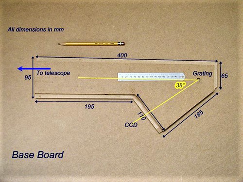
Here’s the base of the spectrograph body indicating the future locations of the grating and detector All dimensions are in mm. The angle between the main optical axis and the diffracted beam reflected to the CCD detector is 38 degrees. This value was obtained using the SimSpec V4 spreadsheet devised by Christain Buil, one of the pioneers in amateur astronomical spectroscopy.
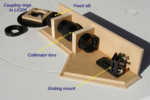
Here’s the spectrograph showing some of the optical components and supports. In this picture I am just playing around with some of the components to check positioning and fit. In order to reduce weight the large 200 mm telephoto was replaced by a simple achromat lens and the collimator focal length was reduced to 150 mm. The fixed slit indicated in this image was eventually replaced by a variable slit (slightly heavier but much more flexible in use).
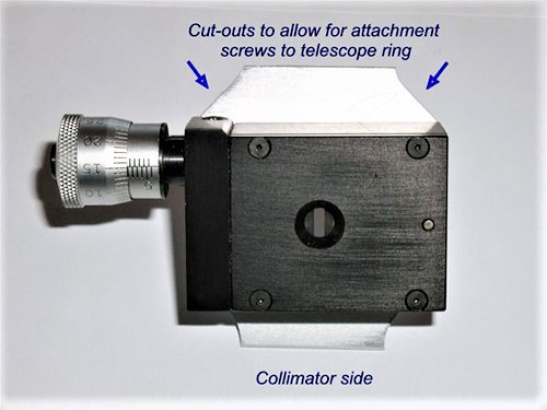
Spectrograph slit seen from the “telescope” side. The metal plate was retrieved from my junk box (conclusion: never throw anything away!) and is used to attach the slit to the rear side of the spectrograph. The corner cut-outs are to allow for attachment screws to pass in order to fix the spectrograph to the telescope.
The slit seen from the “spectrometer” side. An adjustable slit such as this is an important and very useful component, but can be a difficult item to find second hand. This one was retrieved from an old laboratory monochromator, and cleaned up and renovated. Note that a slit such as this can be purchased from specialist suppliers but can be expensive – more than the cost of the whole spectrograph itself! If you cannot find one yourself, a much better idea is to make one from household items such as razor or pencil sharpener blades
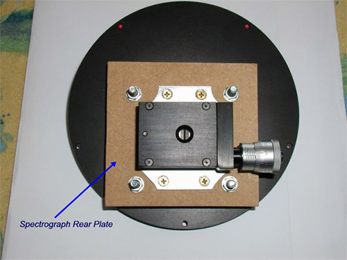
The slit, on its mounting plate, can now be seen fixed to the wooden rear side of the spectrograph during this test. Normally the rear side is permanently screwed and glued to the spectrograph body but is shown here separately for clarity. The large black circular plate comes from an obsolete CCD camera filter wheel that I dismantled. It has the right type of adapter to connect to my LX200 telescope.
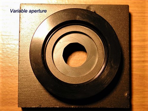
Fitting the micrometer screw into the spectrograph means that a relatively large cut-out of some sort must be made in the side of the body. This could cause some unwanted scattered light to enter, so this variable aperture, mounted in a wooden frame, was used to minimise any stray light. The diameter of the aperture can be adjusted and is usually stopped down to a width just slightly larger than the length of the slit as seen from the grating position.
The beam splitter temporarily attached to its mount with tape. This was originally intended to be inserted between the collimator and grating to allow an off-axis beam to be available for guiding. Since I wanted to test the automatic guiding capabilities of the system, the design called for a portion of the collimated beam to pass through a small video camera lens (adjusted to infinity) that focuses the off-axis beam onto a guide CCD. In the end, the self-guiding capability for the spectrograph was not implemented.
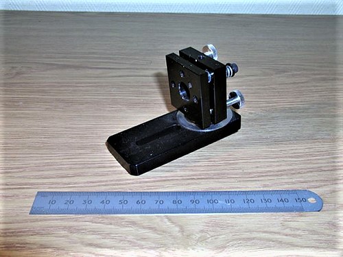
The support mount for the reflection grating. This is a 1.5 inch square mount from Edmund Optics that I attached to a base plate. The mount is also available in a 90 degree version that can easily be fixed to the spectrograph. In my design a 1/4″-20 thread screw passes from the mount base through the bottom of the spectrograph to allow for grating rotation from underneath. Spring loaded adjustment screws on the back of the mount allow for fine corrections if the principal optical axis is not in perfect alignment (which is highly likely with a home-built unit such as this).
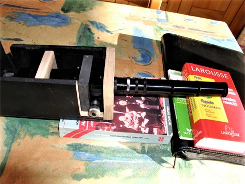
In this, rather strange photo I used all of the coupling rings I could find to simulate an f/10 light cone focused directly on the spectrograph slit. The rings are all connected together to form the long black “tube” with a small collimator lens at the end which has been positioned the correct distance from the slit. This then produces a parallel (collimated) beam from sunlight entering through a window on the right (not shown). The position of this lens is adjusted until the slit image is in sharp focus. In this way, focused light from the slit is then rendered parallel by the collimator when the spectrograph is attached to the telescope which is used mainly at f/10. (My son’s school books were put to good use here in lining up everything!)
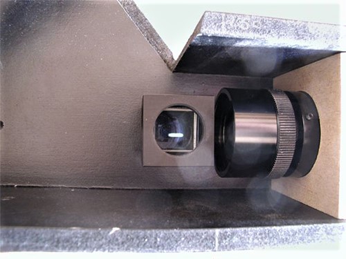
The image of the slit (shown here slightly out of focus) can be seen through the 45º prism placed just after the collimator. A helical focusing ring on the collimator’s lens barrel on the right allows fine adjustments to be made and can be locked in position with a set screw.
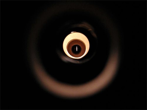
Image of the slit as seen through the access hole that was drilled behind the grating mount at the rear end of the spectrograph. The grating itself is obviously not in position but the grating mount is in position. Fortunately, the mount has a central 8 mm hole that allowed me to check the alignment between the grating and slit positions – my calculations and measurements were OK!
This is basically the same image as above but taken through a small finder scope that has crosshairs. The jaws of the slit can be clearly seen (vertical white line).
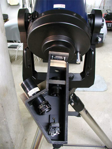
The finished spectrograph, without the top cover, showing its overall size compared to a 12-inch Meade LX200 telescope. Although I made efforts to keep the design as low in weight as possible, the instrument still weighs around 3.2 kg when the CCD camera is included. So some careful adjustments with the telescope’s counterweight system is always required.
Some Example Spectra
Solar Spectrum
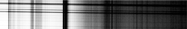
So-called “first light” from this spectrograph is shown in this raw solar spectrum image of the red region. It is the easiest spectrum to obtain from blue sky or clouds. The spectral lines are the vertical lines in this image. The sloping lines running horizontally across the image are caused by light scattered from minute irregularities and microscopic roughness along the jaws of the slit. This can be a common problem but is easily removed during image post-processing. The spectrum is not radiometrically corrected nor calibrated in wavelength. Most of the absorption lines in this deep red region are due to atmospheric H2O and O2.
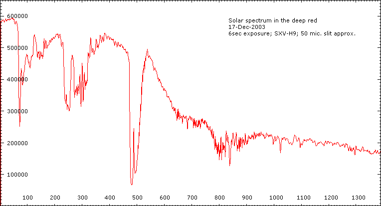
The spectral profile or line trace is shown here, which is the most common method of recording modern spectra. In order to produce this spectrum from the above raw image VisualSpec software was used to take a horizontal line trace from the image and convert to a line profile (regular spectrum). Note that the x-axis on this trace is NOT in wavelength but in pixel numbers and the vertical axis is relative intensity.
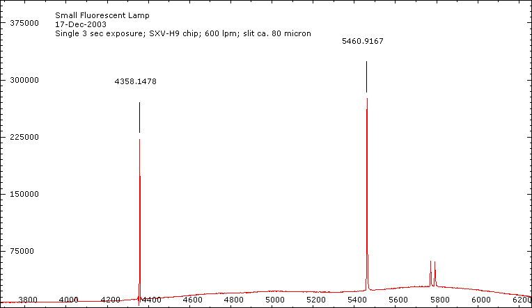
Small Fluorescent Lamp
Raw spectrum image from a small fluorescent lamp showing the dominant mercury emission lines at 436 nm and 546 nm together with the weak 577/579 nm doublet. The corresponding spectrum line trace is immediately below where in this case the x-axis has been calibrated with wavelength in Angstroms.


Pingback: Homemade Spectrometers (Part II) -