If you have been following so far, at this point we should have the Raspberry Pi set up, configured, and the necessary program modules installed.
This final post describes how to upload the data to a website or server.
The simplest way to do this is to create a shell script that the Pi’s command line interface can use.
A shell script is simply a single executable text file with the extension “sh”. It allows you to combine and automate a series of Linux shell (i.e. command line) instructions with a single file. These are executed one by one in sequence, just as if they were executed separately with individual commands.
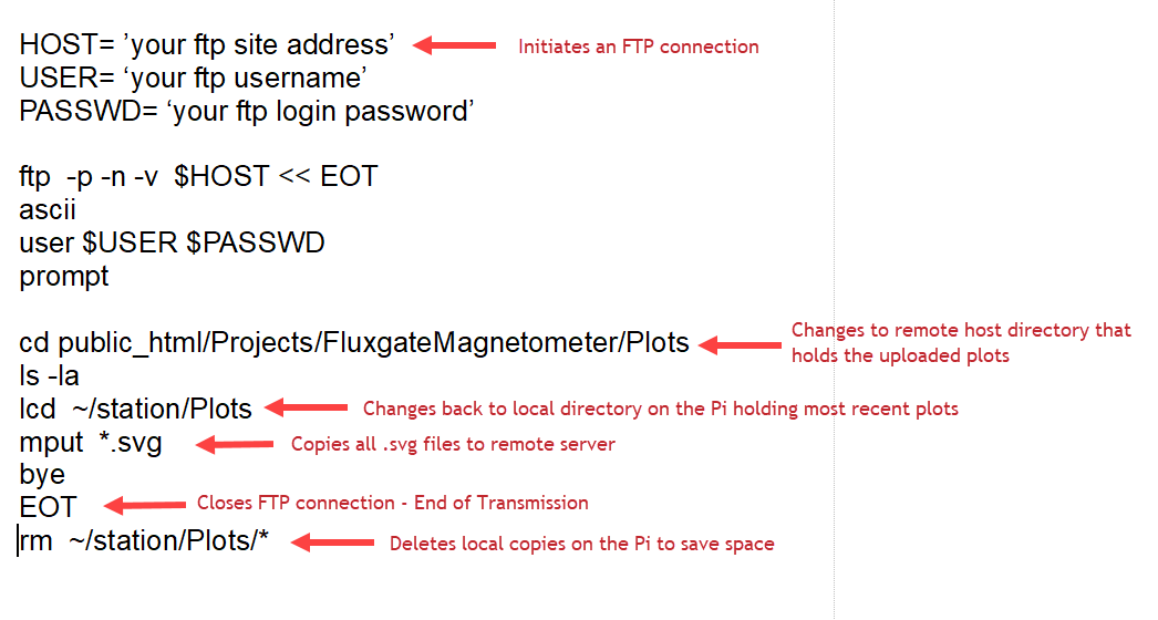
The script given here (courtesy of Ian Robinson again) has been called “uploadHourly.sh” and allows you to send the data to a website every hour and then to visualise the plots on a web page. The script will need to be modified to account for your own FTP address, the password for your web server and site host provider and the folder where you want to save the data.
Here is the script with a few explanations:
Fig. 1
Scheduling the Plots
We are almost there!
The final task is to arrange for the plots to be updated to a pre-defined schedule. This is performed using Crontab.
Crontab stands for Cron Table. Cron is a utility program for task scheduling that was originally developed way back in the 1980’s for Unix-based operating systems. (Remember – Raspbian, Debian, Linux are all derived from the Unix operating system.) The Cron utility therefore schedules repetitive tasks to be run at specific times and dates. This is exactly what we need in order to update our plots.
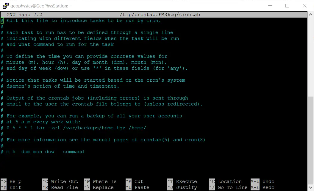
The Cron utility is already part of the Raspberry Pi OS. However, we do need to edit it, in order to add our scheduling instructions. From the Terminal command line, type
crontab -e
This enters the editor, where you see the following screen:
Fig. 2
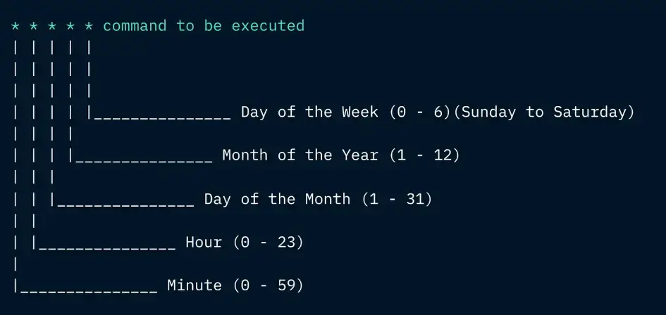
The Crontab data format has to be followed and a simple graphical explanation is shown here:
Fig. 3
As indicated above, the various asterisks are modified according to the time and date schedule that we wish to set. Then the operation to be executed is run.
In the editor window, add the following lines shown in the red box, in the image below, after the last line in the editor’s window. Then save with CTRL-O followed by CRTL-X to exit.
Fig. 4
The first line instructs Crontab to run the uploadHourly.sh file every hour at 2 minutes past the hour. And if there are any errors, to write the errors to the text file called errorsHourly.txt in the station folder.
The second line dictates the actions to take in the event of a reboot. Crontab is instructed to wait 30 seconds after reboot, then to run python3 in the virtual environment and to run the auroraMonitor.py program. Any errors are to be saved as stationErrors.txt in the station folder.
And that’s it. We are finally done with hardware and software setup.
Siting the Fluxgate Sensor
After testing and verifying that everything works, the sensor should be installed in a permanent location which must be as magnetically “quiet” as possible. A spare room in the house is a good choice or down in a basement, garage or perhaps the attic. A corner of the garage may sound like a reasonable choice, provided your don’t have your car in there! One thing the sensor will too easily detect is a large moving metal object such as a car or a metal garage door opening and closing.
The FG sensor is very sensitive. When we consider that the Earth’s magnetic field typically varies from about 25,000 to 65,000 nT during its normal diurnal swings (as explained in Part 1 for this project), and that the sensor will readily detect changes of 1-2 nT, you can see how sensitive this is. So we should expect some random noise in our magnetograms, as well as sudden “step jumps” in our plots, that are often due to moving metal sources in our local environment.
In addition to detecting magnetic field intensity changes, fluxgate sensors are also temperature dependent. As a consequence, the sensor needs to be installed in a place where the temperature hardly (ideally never) changes.
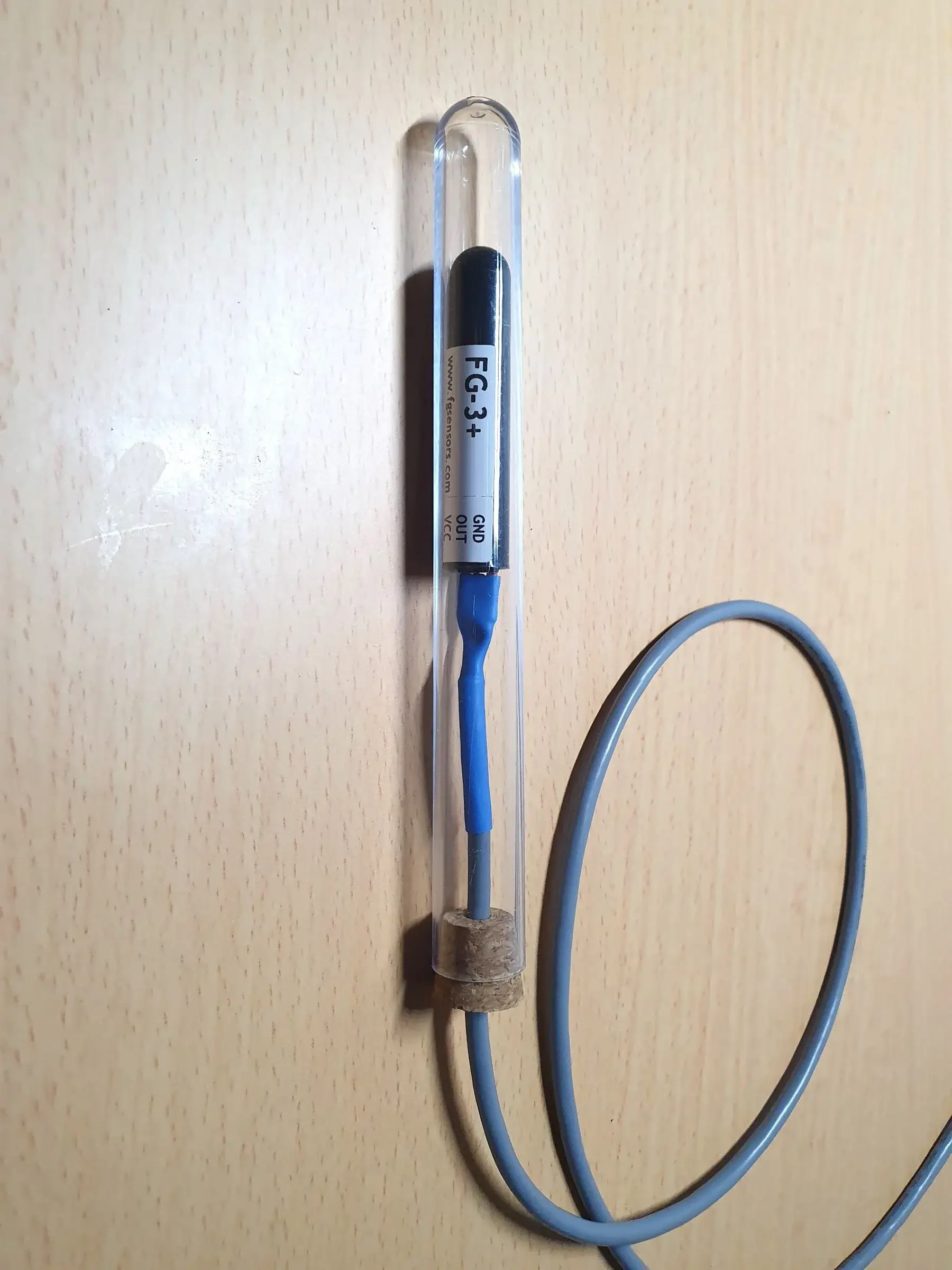
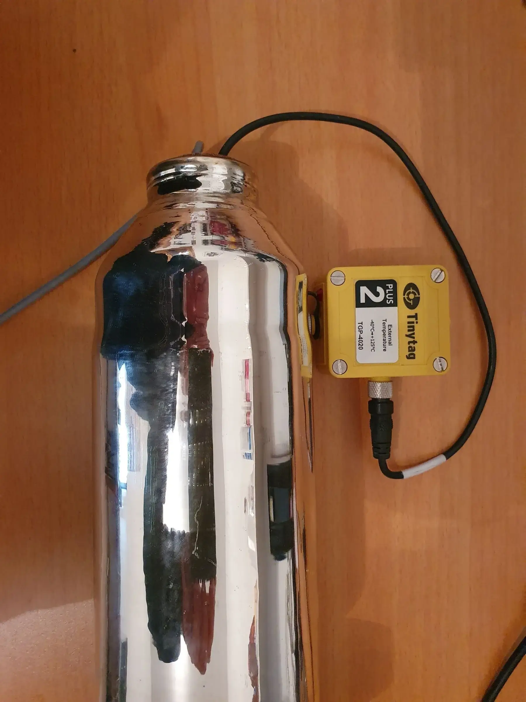
The sensor is located in a plastic tube (shown below) and the tube inserted in a vacuum thermos flask shown in the second image. The flask is filled with polystyrene bead insulation and sealed. The yellow cube is a data logger with a temperature probe in the flask that is used to monitor temperature drift over time.
In professional installations, and also with many amateur setups, the sensor is buried outdoors to a depth of about 1 metre, and protected in some form of moisture-resistant enclosure. Burying the sensor in this way will largely eliminate daily changes in temperature, but it may not completely eliminate any long-term seasonal drift.
In some professional installations, the magnetometer and associated electronics are kept in a temperature controlled enclosure or even a whole room.
It should be noted that it is only the changein temperature that will cause the sensor output to vary. The actual temperature itself is relatively unimportant, as long as it remains constant.
This setup will be left running for a few months to monitor temperature stability inside the thermos flask. If this proves to be inadequate, the option to site the sensor underground as mentioned above will then be considered. More information on a sub-surface installation is available at this link which investigates sensor burial depth and its effect on reducing natural temperature variations.