Introduction
Well, it has taken me a few months to get around to finishing this particular project, but here are the final sections that I have split into two parts.
In the Part 1 and Part 2 articles, we covered the basics of the fluxgate magnetometer (FGM). We explained how it can be used to monitor solar activity and the possibility of you seeing an aurora. If you have been following this project so far, and constructing this magnetometer, we should now have the Arduino recording frequency pulses from the FG Sensor.
In Part 3 here, I explain how to connect a Raspberry Pi to the system. The Pi will process data coming from the Arduino, will generate the magnetometer plots. The final Part 4 then describes how to upload the plots to a web site, plus some ideas on siting the magnetometer. Setting all this up can be somewhat involved, so things have been broken down into several small steps with images to guide you.
First of all, a few words concerning the Raspberry Pi.
Which Raspberry Pi?
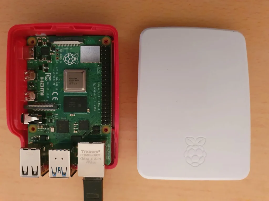
Unlike the Arduino, which is essentially a ‘bare bones’ microcontroller, the Raspberry Pi is a fully-fledged minicomputer in its own right. And like the Arduino, the Pi has a very large fan community that was described in a previous post. The Pi comes with USB, Ethernet and wireless support, a high capacity memory card slot, and connections for a mouse, keyboard and HDMI port for a monitor. All this installed on a small printed circuit board (PCB) not much larger than a credit card!
There are several versions of the Pi. My first one, purchased over 10 years ago, was a Raspberry Pi 3 Model B. These were immensely popular at the time, and the Pi 3 still performs very well. However, things have moved on technologically. For this project, I would recommend that you go for the Raspberry Pi Model 4, which is much faster and has more functionality. Prices do increase with the amount of RAM that you want, but for this project 1-2GB of RAM is vastly more than you’d ever need.
Setting up the Pi
Some parts of this next section, especially the installation of ObsPy (see later) borrow information supplied to me by Dr. Ian Robinson at Starfish Prime, to whom I am most grateful for assistance in getting my own system up and running correctly.
1. The Operating System
First of all, we need to install the operating system (OS). The Pi uses an OS called Raspbian. (The folks at the Raspberry Pi official site recently renamed their OS and now refer to it as “the Raspberry Pi OS” instead of Raspbian. Not very original, in our opinion, so we are still going to stay with Raspbian for this project. We just like the name!)
Raspbian is a version of the Linux operating system called Debian and the latest 64 bit version is V11 and is codenamed Bookworm. This is the OS we will be using. Full details on how to install this OS, complete with video tutorials, are available here and software for installing Raspbian, on a Mac, Windows or Linux computer is available here.
The easiest way to install the OS is to download the Raspberry Pi Imager program. This is shown on the RPi site here:

The Raspberry Pi Imager application downloads a complete image of the whole Pi OS onto your PC. It is available for Macs, Windows or Linux machines. This is then transferred to an SD memory card for use with the Pi. So you will need an SD card reader. Many PC’s have these, but if your desktop or laptop does not come with one, they can be bought for just a few $/£/€.
Run the Imager program. The latest version of the Pi Imager prompts you to customise and preconfigure the OS before it is flashed to the memory card, as shown here:
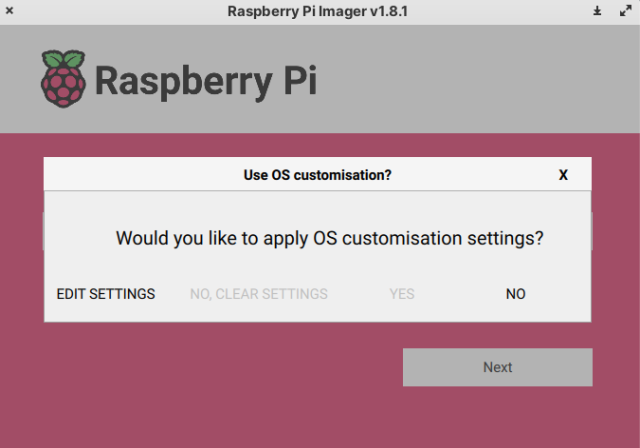
Click on “Edit Settings”, which takes you to the Customisation Window with three panels: General, Services and Options, shown here:
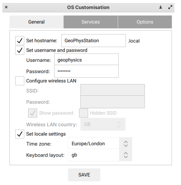
Set a hostname. I have called this “GeoPhysStation”, since I may be using this Raspberry Pi with other geophysics sensors in future, in addition to the current fluxgate sensor for this magnetometer project.
Similarly, the username has been called “geophysics” and a password set. Change the locale and keyboard settings as required for your own location. Mine has been changed to Europe/Paris with “US” as the keyboard layout which is different to Figure 4.
Under the Services tab, enable SSH. SSH stands for Secure Shell, or Secure Socket Shell. It is a network protocol that provides users with a secure way to connect to a computer over an unsecured network. So enabling SSH allows us to log in to the local network securely.
Then click “Next”, and the Imager program should start to write the OS image to the SD card. This takes a few minutes, depending on the speed of your PC, so go and grab a coffee.
The SD card can now be removed from the PC and inserted into the Raspberry Pi.
2. Booting your Pi - Headed or Headless Mode?
Now there are two ways to go about booting the Raspberry Pi. The usual way is called headed mode. This is where we connect a mouse, a keyboard and a display monitor, exactly as we would with any other desktop computer, regardless of size – recall that a Raspberry Pi measures less than 10 cm x 6 cm!
The other way is called headless mode. This is where we communicate with the Pi using another PC, such as a laptop, over a network connection and use the Pi’s Ethernet port to talk to the PC.
Headed mode is obviously the more familiar to most of us, and is very convenient, especially if you have never used a Raspberry Pi before. But eventually, when the project is finished, everything is set up, and data from the fluxgate sensor are being recorded and processed, headless mode is best. This is because it avoids you having to devote a keyboard, a mouse and a display full time to the system. All that is needed is a network connection.
And once installed, the Pi can be left running for months, without any intervention, provided the network connection is stable. So with this project, we are going to use Headless Mode.
The easiest way to connect your Raspberry Pi in headless mode is by employing a free SSH client and terminal emulator, of which there are several available online. One of the most popular is PuTTY, which can be downloaded here. When you launch PuTTY from your PC, you are presented with this interface:
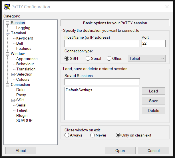
Type in the host name that you created when customizing the Pi OS (in my example this was “GeoPhysStation”, then press “Open”. You will be asked for a password. Use the same password you created during the OS customization. This opens the SSH connection and presents you this window:
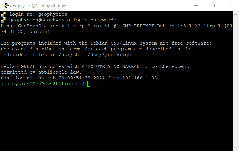
This is the command line window. We are now connected to the Pi over a secured network connection. The next sections will be using some Linux (Debian) commands. For readers unfamiliar with Linux, just type in the relevant commands and follow along. There are many online sites that explain the most common Linux commands that you can read about.
3. Configuring the OS
At this point, we have installed the OS for the Pi, and are communicating directly with the Pi through our PC and the terminal emulator PuTTY. We now need to configure the OS. At the command line in Figure 6 above, type
sudo raspi-config
This opens the Pi’s Software Configuration Tool:

Select 1 (System Options) which opens the following window:
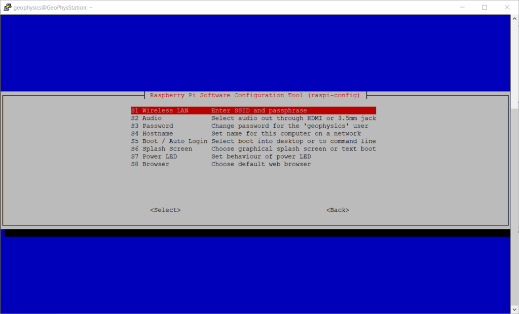
Then select S5 (Boot / Auto Login) to bring up the following options:

We have a choice at this stage. The best two options are B2 or B4 which automatically log us in as the “geophysics” user, which is what we want.
For a basic command line console, select B2. With B2, once we have saved the configuration and rebooted the Pi, we should see the simple command line interface (terminal window) from which we can type in our various commands.
However, if you are more comfortable with a desktop style display with browser, wastebasket, terminal, and all the other icons and menu options, then select B4. After reboot, you are presented with the standard Pi OS desktop, from which you can also access the Terminal console.
Back at the home menu of the Configuration Tool (figure 7) select Advanced Options followed by A1. This will expand the file system to ensure that all available space on the SD card is used.
We can now exit the Configuration Tool and then reboot the Pi with the command
sudo reboot
From now on in this project, I will assume that we have a fully functional Raspberry Pi with Raspbian loaded, any updates and security patches have been installed, and the OS is functioning as it should.
4. Installing the Required software
Install the following series of routines, either by opening the Terminal from the desktop interface or from the command line.
Install FTP
FTP (File Transfer Protocol) is a standard means to transfer files from a local machine (your PC) and a remote host (such as a web server). There are free FTP programmes that do this. Your website host provider may recommend you to use specific software for FTP and if so they should have instructions on how to upload files on their hosting site. A very popular one that many host providers use is called FileZilla.
From the command line (either using PuTTY or using Terminal from the desktop interface) install the FTP routine on the Pi with the command
sudo apt install ftp
Set the Time
In order to ensure that the time axis on our magnetometer plots is accurate, we need to install NTP, which stands for Network Time Protocol. NTP is used by hundreds of millions of computers every day to synchronise their clocks over the Internet. They work in the background of course without you realizing it.
Install NTP with the following command:
sudo apt install ntpdate
Then activate the NTP routine with the command:
sudo timedatectl set-ntp True
Note: One thing to bear in mind is that the Raspberry Pi will be retrieving the correct time from the Internet. Unlike most other desktop and laptop computers, the Pi does not have an internal clock of its own. So if your internet router goes down temporarily for any reason, the time data added to the plots may not be correct.
A solution to this is to add a Real Time Clock (RTC) module, (although this is entirely optional for this project). The RTC module connects directly to the board of the Pi. These modules only cost a few dollars and full details on how to do this can be found here.
Install the ATLAS Maths Package
ATLAS stands for Automatically Tuned Linear Algebra Software. It is a required maths package for our data to be processed correctly. Install it at the command line interface with:
sudo apt install libatlas-base-dev
Install ObsPy
ObsPy is central to the set of programs that we are installing here, since it is used to generate to plots from the fluxgate magnetometer data. ObsPy is a collection of open-source software routines & libraries. As the second half of the name implies, it is written in the Python programming language. (Don’t panic; no previous knowledge of Python is required to get things to work!)
ObsPy’s suite of routines is more or less standardized for processing time-series data from geophysical instruments such as seismometers, magnetometers, infrasound detectors and similar sensors.
Contained within ObsPy is miniSEED. This is a data format that we shall use to produce our live magnetometer plots. SEED stands for Standard for the Exchange of Earthquake Data and miniSEED is a stripped-down version of this program without all the metadata.
In order to install ObsPy and have it work correctly with Python interpreter, it is best to create what’s called a virtual environment – the reasons why are explained in more detail later.
Usually, Python will already have been automatically installed system-wide (as python3) when you installed the Raspbian OS. To install a virtual environment, at the command line interface in terminal mode, type the command
sudo apt install python3-venv -y
(Again, if you don’t know much about Debian (Linux) commands, don’t worry. Just type in the exact commands, including any spaces, word for word. There are many online sources listing the most common Debian terminal commands for anyone interested.)
Then create a folder that will contain our python3 virtual environment with the command:
python3 -m venv ~/my_venv
If we then list the folders with the ‘ls’ command, we should see something like this in the folder list in blue, showing that our virtual environment folder (that I have called ‘my_venv’) has been created correctly:

Now we activate our newly created virtual environment with the command
source ~/my_venv/bin/activate
When we do this, the command line prompt becomes prefaced with the name of the new environment (that I called my_venv) as shown by the red arrow here:

We now have a working virtual environment into which we can install ObsPy, using the command:
pip install obspy
Installing ObsPy does take some time so we can go and have another coffee.
Why a Virtual Environment?
So why did we go to all the trouble of creating a virtual environment just now?
One potential problem we can meet is that ObsPy cannot be directly “unpacked” by the latest version of the Raspberry Pi’s OS. This latest version of Raspbian (codenamed Bookworm) now has an additional security feature that considers the ObsPy suite of programmes to be a non-official software package (most probably because it is open-source). So when you try to install ObsPy system-wide, as we would normally do, we can run into problems. The installation fails, which was my own experience on the first attempt!
Fortunately, there is a workaround… we create a local version of Python, specifically for our magnetometer project, and install ObsPy into a virtual environment that our local Python installation can then recognize and work with.
The potential issue that can arise comes from version updates. Versions of Python3 are updated regularly, whereas Obspy, being Open-Source software, is updated only occasionally and infrequently. As a result, versions of Obspy can “lag behind” the latest Python version and installation package dependencies can break during your Obspy install. So the installation fails. To use a term from Dr. Ian Robinson at starfishprime.co.uk, “we risk entering dependency hell”.
To avoid this, we set up a second local Python install in a virtual environment, where we have also installed Obspy. Using the pip installer, we ensure that the local version of Python and ObsPy match. To quote Ian again, the result is “dependency heaven”.
One final thing to be aware of is that when the command “source ~/my_venv/bin/activate” was issued above, we instructed the terminal program always to run the local version of Python, and not the system-wide version. This activation of the virtual environment unfortunately ends when we logout or reboot.
Therefore we must remember always to call the local version explicitly (and not the system-wide version) whenever we launch a Python program that needs ObsPy, such as the monitoring program that we will require.
Install the required Communication software
Next install the following communication routines with the commands:
pip install smbus2
pip install serial
smbus2 is used by the monitoring program (see later) and serial is needed for the Pi to communicate with the Arduino microcontroller that is receiving the data signals from the fluxgate sensor, as explained in the Part 2 of this project.
Install the Monitoring Program
Create a new folder (which I have called ‘station’) from the Terminal window with this command:
mkdir station
Upon its first run, this will automatically create subfolders for data and plots. Using FTP from the command line interface, (or ‘drag-and-drop’ if you are using the Pi’s desktop interface), copy the monitoring code to the station folder.
Three files are required:
- geostationModules.py
- globalvariablesModule.py
- auroraMonitor.py
auroraMonitor.py is the sensor-specific monitoring program for this project. Others are availaabe for different sensors such as a microbarometer (infrasound) detector. All of these program modules are courtesy of Dr. Ian Robinson, used with permission, and are available at this link. For more information go to the starfishprime site.
The final post in this project explains how to upload the files to a website and (briefly) where to site the fluxgate sensor.
