Introduction
The humble Bunsen Burner has been a ubiquitous piece of lab equipment ever since it was invented by the German chemist Robert Bunsen in 1855. A testament to its great success is that this very simple and efficient device still continues to be used in science teaching and research labs all over the world.
The structure of the Bunsen burner flame, and the colours it produces, depends on how the burner is fed with fuel and air. In particular, how much air is allowed to enter the burner tube, via an air intake, before combustion takes place. This air inlet is usually adjusted with a metal ring, as can be seen here in this modern version of the burner:
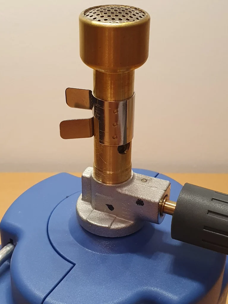
Since my home is not connected to any public gas network, I am unable to produce a flame with regular town gas and a standard burner. So the next best thing is a camping gas stove and canister, with a Bunsen adapter, as you see in the above image. The gas supplied is a mixture of the hydrocarbons propane and butane.
If the air inlet is fully closed, the burner flame is described as “fuel rich”. The flame burns with a bright yellow sooty flame and the general spectrum is continuous. Microscopic black carbon particles glow yellow to incandescence and black smoke from the particles is easily observed at the top of the flame. Under these conditions, the ceiling of any experimenters home lab can rapidly become stained black if you are not careful. Take my word for it!
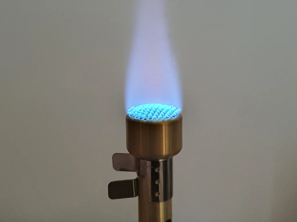
When the air inlet is completely open the burner is considered to be fully pre-mixed with air before combustion takes place. Under these conditions the Bunsen burns with an almost invisible blue-green flame. It is this state that is of most interest to amateur experimenters, both chemically and spectroscopically. The hottest part of the flame is just above the electric blue coloured zone shown in the image below.
The invention of the Bunsen burner arrived at the perfect time in the mid 19th century when physicists and chemists began to investigate the emission spectra of elements and other materials when heated to incandescence. A few years after the invention of his burner, Robert Bunsen again struck gold when he collaborated with the German physicist Gustav Kirchhoff that led to the invention of the prism spectroscope in 1859.
These two inventions, Bunsen’s burner and the Kirchhoff-Bunsen spectroscope, when used together, proved to be the keys to a greater understanding of light emission from the elements. As a consequence, the new and vitally important field of spectrum analysis was born.
The Swan Bands
Although you may not realize it, the Swan bands are seen by practically everyone who turns on a gas cooker every day to brew a cup of tea. The bands are also seen by welders who use oxyacetylene torches as well as chemistry students using Bunsen burners in their lab classes. The Swan bands have also been detected in certain comets, in the interstellar medium and in late type white dwarf stars that are known as carbon stars.
The Swan bands are a group of molecular spectral features, occurring mainly in the blue-green region of the visible spectrum. Today the bands are well understood to originate from the emission of light from two specific electronically excited energy states of the diatomic carbon molecule, which is also called dicarbon or C2.
But back in the mid-19th century, when these bands were first observed, it was an entirely different story…
These strange emissions were first discovered by the Scottish physicist William Swan in 1856, and the exact nature of the chemical species producing the bands was far from clear. This spectroscopic puzzle led to a fascinating and prolonged scientific debate that lasted well over 40 years, with arguments and counter-arguments proposing different hypotheses along the way. Today, they are still known as the Swan Bands in honour of Swan’s original discovery and his efforts in this nascent field of emission spectroscopy.
As mentioned above, the Bunsen burner had just been invented two years earlier. Although chemists and physicists had begun to experiment with dispersive optics and prisms to examine the properties of light emitted when elements were heated, the invention of the classical spectroscope was still a couple of years away.
To pursue his investigations, Swan used a flint-glass prism that he had acquired from the Swiss optical instrument maker Marc Secretan, who was based in France at the time and working at the Observatoire de Paris. Together with a theodolite (of all things!) that was a loan from a Mr. John Adie and a Professor Forbes, these items enabled Swan to disperse the light from a sample gas flame into its constituent wavelengths and to measure the different angles of deviation exiting the prism.
Swan employed a variety of gases in his studies that he called “carbohydrogen” flames. By carbohydrogen, he essentially meant hydrocarbon gas (molecules containing carbon and hydrogen atoms) although he did include some compounds containing oxygen in his experiments.
Swan presented his data in units of deviation angle, which at the time was a common way to measure the dispersion of light through prisms. Fortunately, he had the insight to record simultaneously the deviation angles from the well known Fraunhofer lines seen in the solar spectrum, whose positions (wavelengths) were known fairly accurately at the time. So it was a simple matter to convert the angles into wavelengths.
Assisted by similar investigations of flames by his contemporaries Sir William Davy and John William Draper, Swan was well aware of the basic physical structure of the flames (“sooty” and “clean”) and their changing emission characteristics and appearance. But Swan went further to pursue, in some detail, the nature of the chemical species of various heated materials using the newly invented Bunsen burner and coal gas as a fuel source.
Swan examined a wide variety of hydrocarbon samples in his work, ranging from “light carburetted hydrogen” (which we now call methane) and “olefiant gas” (now called ethylene or ethene). What was curious was that the positions of the spectral bands observed in all of these samples were, in every case, practically identical !
So Swan investigated further and examined the emission spectra of heavier (higher molecular weight) hydrocarbons. Samples of paraffin oils, oil of turpentine and compounds of more complex chemicals such as simple alcohols and ethers, tallow wax and camphors, were all examined and described in Swan’s published work. Fascinatingly, the results were always the same: the visible emission band spectra, in almost every case, were essentially identical.
This critically important observation suggested that some overall common chemical entity was being produced in the combustion process that was producing these rather mysterious spectral bands.
But what was this strange substance?
The Dicarbon Puzzle
Dicarbon. It sounds like some mysterious new element or some exotic new material from Star Trek. But whereas the Starship Enterprise’s Dilithium crystals are pure fiction (with my apologies to all you Trekkies out there), dicarbon is a very real molecule, albeit a rather transient and highly unstable one.
When William Swan first observed these bands in his carbohydrogen flames, he not unreasonably attributed them to some form of hydrocarbon species. After all, the samples that he tested all contained the elements carbon and hydrogen. He labelled the bands with the Greek letters alpha (α) through zeta (ζ) in his early published work.
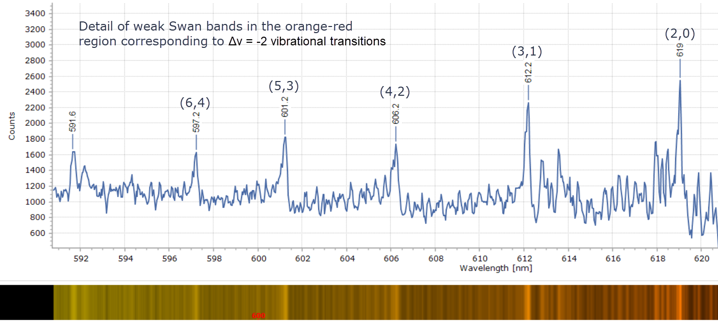
A low resolution spectrum of the Swan bands across the visible spectrum can be seen in Figure 3. These bands appear in clusters from the blue to the red and I have attached Swan’s own labels (α, β, γ, etc.) that he gave to these bands in his original paper.
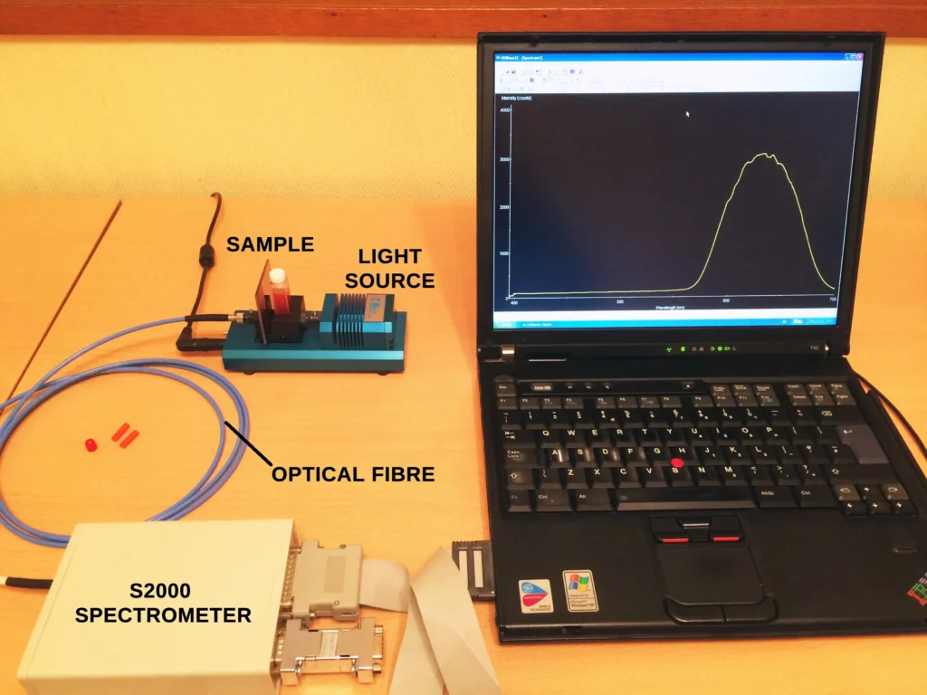
This spectrum was obtained in my home lab with a 100 micron optical fibre placed close to the exact same Bunsen flame shown in Figure 2. Light from this source was then fed into an Oriel Newport MS125 1/8th metre spectrometer with a 600 lpm grating and an Andor iDus 420 CCD detector.
Here is the result…
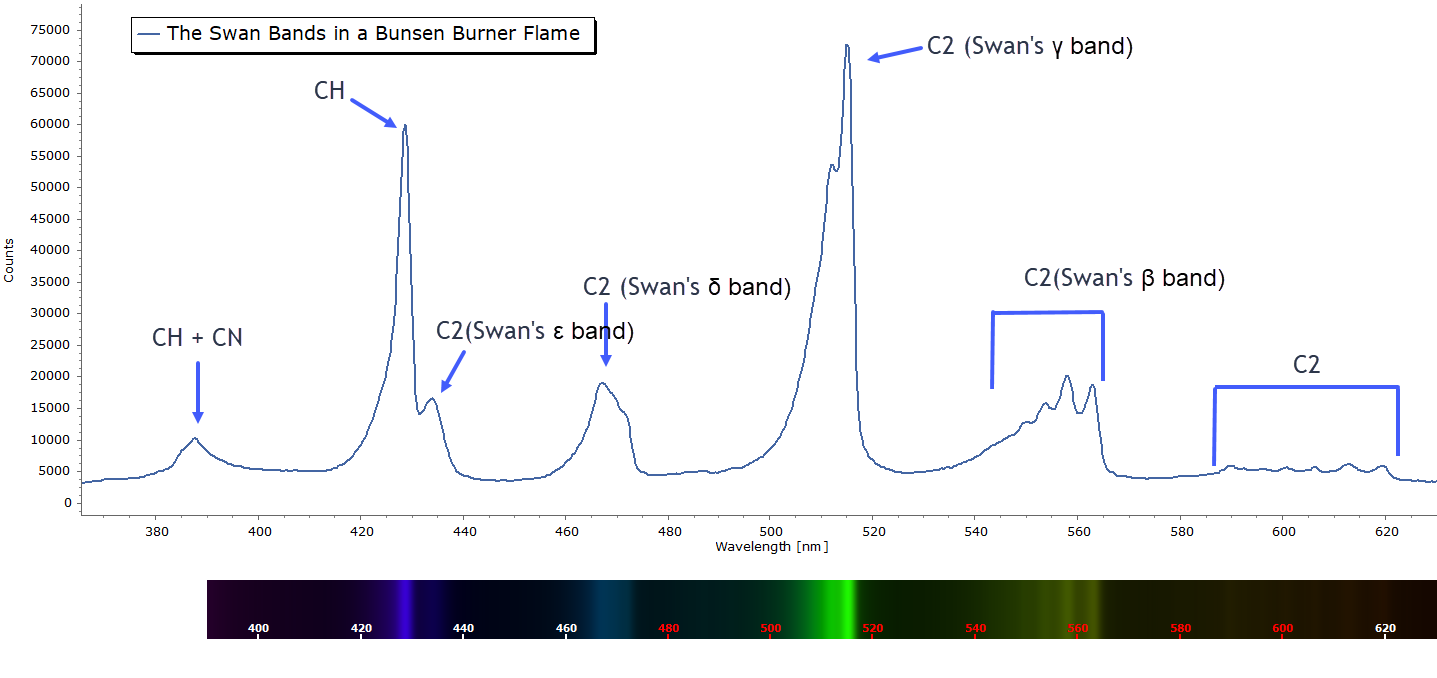
Note that there is no “alpha α band” in the spectrum above. Swan’s equipment was probably not sensitive enough to detect the weak bands actually seen around 600 nm in the red region. Nevertheless, these weak bands are also due to C2. A sharp line that Swan did report as ‘α’ in his original paper is almost certainly due to sodium, since it corresponds to the Fraunhofer sodium D line seen in the absorption spectrum of the Sun at 589 nm. It was most probably observed due to some contaminant in the gas stream that Swan was using.
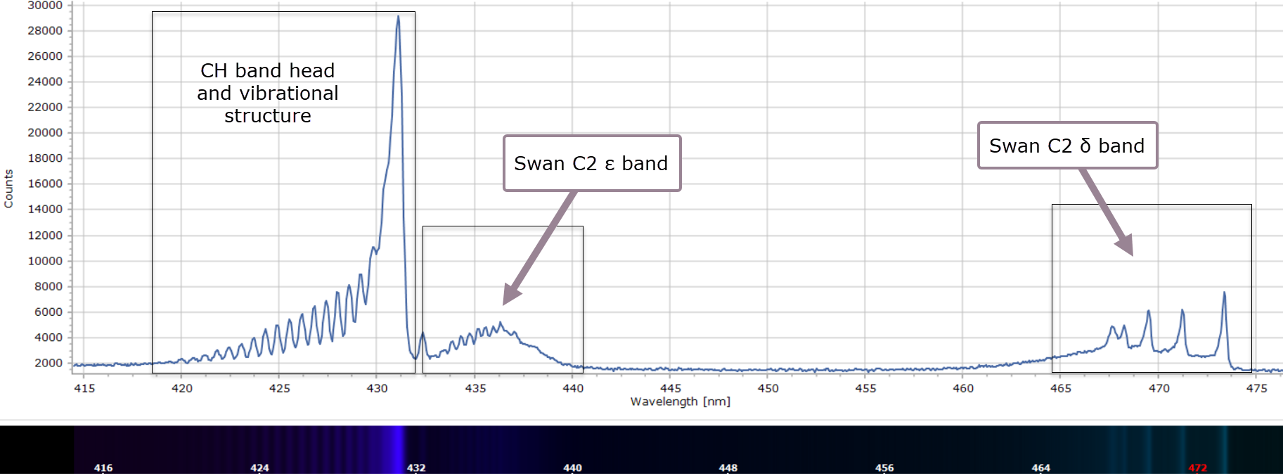
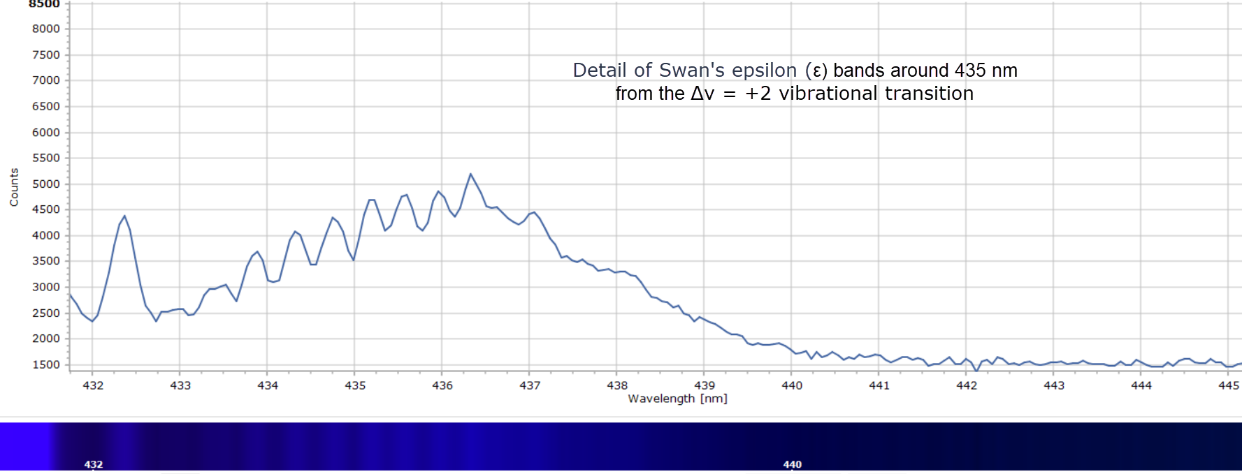
Consequently, there is no alpha line in the spectrum in Figure 3, which was obtained from a clean, pre-mixed flame of a butane/propane gas mixture (a Campingaz™ Labogaz 206 canister). There is, however, a strong band at 431 nm that Swan did observe and labelled ζ. This is not due to C2 but is actually from the methylidyne radical, CH. And around 388 nm, in the violet region, are bands due to CH and CN radicals.
Nonetheless, the groups that Swan called β, γ, δ and ε are indeed the four principal emission bands that are today recognized as vibronic (vibrational-electronic) energy transitions from the dicarbon molecule C2. Today they are recognised as the Swan Bands in honour of his discovery.
However, the actual chemical nature of all these bands, and why they appeared in clusters with some tantalizing underlying structure, still remained unclear and elusive at that time…
Enter John Attfield, the first scientist to assign the Swan bands to diatomic carbon, C2. Interestingly, Attfield was an accomplished pharmacologist by profession. In the summer of 1862 he had been appointed Director of the Laboratories of the School of the Pharmaceutical Society of Great Britain. But Attfield had a more than passing interest in spectroscopy and became interested in the C2 puzzle.
In that year Attfield’s original research in this field was read to the Royal Society of London in a paper called “The Spectrum of Carbon”. (In those days, if you were not a member of this very distinguished society, your original work had to be read out to members of the society by a scientist who was already a member! Perhaps this is still the case today, but I would need to check.)
Now we know that Swan considered the bands to be due to some type of hydrocarbon, the two essential components being carbon and hydrogen atoms in his carbohydrgen flames. But Attfield challenged this interpretation. He showed experimentally that exactly the same bands could be seen in the combustion of the gas cyanogen (CN)2, which at the time was produced by the thermal decomposition of mercuric cyanide. Attfield went on to observe the same identical bands in electrical discharges of carbon monoxide (CO) and also with carbon disulphide (CS2).
Attfield argued that since none of these compounds contained hydrogen atoms, and because the only common element they contained was indeed carbon, these spectral features must originate from some form of elemental carbon. The common denominator was carbon.
In the years that followed, Attfield’s “carbon theory” began to be accepted by most spectroscopists. But then in the 1870’s, it was challenged by the great Swedish physicist Anders Jonas Ångström (from whom we have the Ångström unit of wavelength) and his colleague Robert Thalén, in a paper, originally in Swedish and published in 1875, a year after Ångström’s death. Ångström and Thalén thought that Swan’s carbohydrogen bands must be acetylene C2H2.
Their justification was based on experiments with different gases in spark tubes that had pure solid carbon electrodes to create a discharge. With hydrogen in the discharge tube, the Swan bands appeared. When the gas was changed to oxygen, carbon monoxide bands were observed, and when nitrogen was tried, bands due to cyanogen (CN) were seen. Reinforced by Ångström’s very distinguished reputation (he was considered one of the founding fathers and doyen of spectroscopy), this became known as the “acetylene theory”.
As a consequence, scientific opinion began to swing back to Swan’s hydrocarbon proposal.
Now Attfield could never be entirely sure that moisture (and therefore hydrogen) was totally absent in his experiments. At that time it was experimentally very difficult to ensure that all moisture had been purged from his equipment. This turned out to be a weak link. Attfield was forced to admit that the Swan bands he observed “could in principle” be due to hydrogen impurities and therefore not due to C2.
And so the arguments against, and the challenges to, the carbon theory continued once more, with the pendulum of scientific opinion swinging back to hydrogen and the acetylene theory.
It was around this time that band spectra were beginning to be generally accepted by chemists and physicists as being molecular in origin, whereas narrow line spectra were understood to originate from atoms. Furnished with such knowledge, the spectroscopist W. Marshall Watts came to the defense of Attfield’s conclusions in 1875 when he asserted that “The [Swan] spectrum … is a spectrum of the first order [i.e. a band spectrum] and [therefore] the spectrum of a compound. If however the spectrum be caused by a compound it can only be a compound of carbon with carbon.”
Be that as it may, the debates and objections continued unabated. It must have been difficult for chemists to accept the idea that carbon (i.e. graphite), considered to be one of the most refractory of materials, could be formed in the vapour phase and then emit light. The counter argument to this, of course, was that carbon could be formed in the gas phase relatively easily by decomposing any volatile organic compound!
It appeared to be a stalemate, between the carbon theory on the one hand and the acetylene theory on the other.
And this impasse continued until improved instrumentation and, just as crucial, a better theoretical understanding, was developed and subsequently verified by experiment.
Both of these advances came along slowly over the next 40-50 years
The story of this, at times rather polemical, debate is recounted in J. C. D. Brand’s excellent book “Lines of Light: The Sources of Dispersive Spectroscopy, 1800-1930” which is a very entertaining history of early prism spectroscopy and the new field of spectrum analysis. Besides the Swan band arguments, this fascinating work describes many more descriptions and anecdotes of the problems facing chemists and physicists during this evolutionary period. Many of these scientists were somewhat colourful characters, with very strong opinions and reputations to defend and uphold.
A highly recommended work to any interested reader willing to make the effort!
So in conclusion...
To bring this brief historical account to something of a conclusion, by the 1920’s improvements in prism spectrometers that could take long exposures of spectra on sensitive photographic plates began to produce some extremely detailed information on the controversial Swan Bands, and their so-called band heads or band edges.
The actual significance of these features only began to be appreciated with parallel developments in the theory of optical spectroscopy and a much better understanding of molecular band spectra. In particular, the development of quantum theory and quantum mechanics in the 1920’s and 30’s, as it applied to the spectra of diatomic molecules, played a vital role here.
These advances ultimately led spectroscopists finally to accept that the Swan bands do indeed originate from the emission of visible light from the dicarbon molecule, C2.
The Swan Bands at higher resolution...
The Swan band spectrum produced in my home lab in Figure 3 shows the band clusters in low resolution across the complete visible spectrum from about 400-600 nm. Even so, some tantalizing detail and structure appear to be just under the surface.
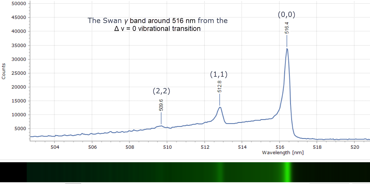
When each cluster is recorded at higher resolution, using a 2400 groove per mm diffraction grating, fascinating detail of the vibrational fine structure within the bands reveals itself in Figures 4 – 9 below.
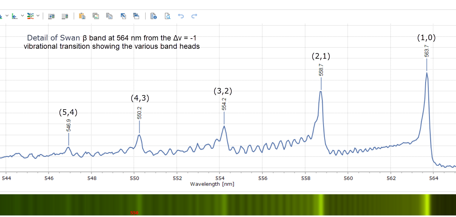
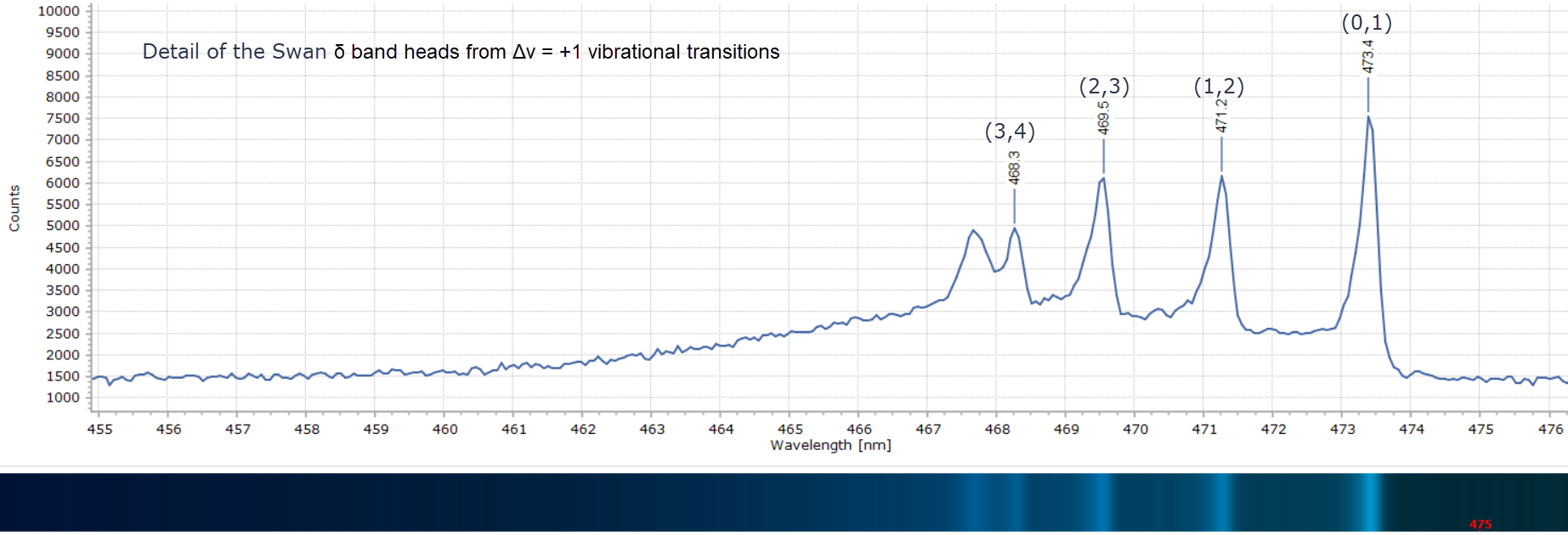
The peak maxima are labelled in wavelength (nm) and the modern vibrational assignments – the numbers (x,y) – have been included. This is spectroscopic terminology representing the vibrational quantum number, v. By convention, v’ is used to denote vibrational levels of the upper electronic state, and v” denotes those of the lower electronic state. As an example, if the bands are labelled using the convention (v”, v’) with the lower state written first, then the set (1,0), (2,1), (3,2), (4,3) and so on forms a sequence with Δv = -1. This is what we see in Figure 5 with the Swan β bands. These features are indeed called sequences in the jargon of spectroscopy. Other spectra are labelled the same way.
Final Words...
The chemical mystery surrounding the nature of the Swan bands has been solved now for well over 80 years. All arguments to the contrary have finally been put to rest.
Fascinatingly though, what is still very much a subject of discussion and research, even in today’s modern times, is the exact nature of the chemical bonds that hold the two carbon atoms together in this rather strange diatomic molecule.
But that would be a whole new topic of discussion that could require several chapters to do it justice. Or even a whole book!
References
- Swan, W. (1857) Trans. R. Soc. Edinburgh., 21, 411 – 429.
- Gaydon, A.C. (1974) The Spectroscopy of Flames, 2nd edn. Chapman and Hall, London.
- Attfield, J. (1862) Phil. Trans. Roy. Soc. Lond., 152, 221 – 224.
- Ångström, A.J. and Thalén, R. (1875) Nova Acta Reg. Soc. Sc. Upsal., 9.
- Brand, J.C.D. (1995) Lines of light: The Sources of Dispersive Spectroscopy, 1800 – 1930, CRC Press.
- A. Tanabashi et al., (2007), Astrophysical J. Supplement Series, 169, 472-484.
The introduction took me back to 1964/1965, and introduced me to the idea that science isn’t always exact.
My first secondary school was in Grimsby and naturally enough the Bunsen Burner featured in one of the first Chemistry lessons, if not the first. The fame was described in 3 stages according to how much the collar controlling the air was opened. Visible, invisible and finally roaring when it was fully opened.
Nine months later we moved to Burnley and to cut a long story short, I started in a new school but again in the first year. (It was also when I met Stephen). Again the Bunsen Burner made it’s appearance, but here it only had 2 states, Visible and invisible. The Bunsen burner didn’t roar again!
A very informative read 🙂