Modern spectrometers today, regardless of their size, employ sensitive linear CCD and CMOS sensors. The most popular sizes have 1024, 2048 and more recently 4096 pixels along the dispersion axis of the grating. Associated software automatically reads out a series of digitized values, each value corresponding to a single pixel element on the detector.
So once acquired, the spectral data are already in the form of signal intensity up the Y-axis and pixel value along the grating dispersion X-axis. It is usual, however, to convert the horizontal axis into the more meaningful units of wavelength (λ) and this becomes absolutely essential when spectral line identification of an unknown sample is the objective.
Wavelength Calibration
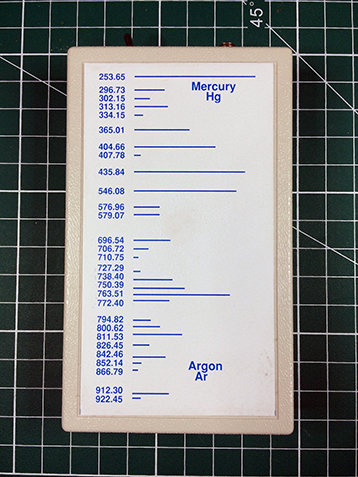
I will use the MS125 spectrometer as an example of the procedure. This spectrometer has interchangeable gratings and a micrometer screw to change the wavelength range. A fresh calibration must be performed when a grating is changed or the micrometer setting is adjusted. What we are doing with this procedure is mapping every pixel number on the linear array sensor to a specific wavelength and this is best performed with spectral calibration lamps that have very narrow emission lines whose wavelengths are known very precisely.
Kr and Hg(Ar) Spectral Calibration Lamps
The relationship between pixel number and wavelength can be expressed as a third-order polynomial of general form
λp = I + C1p1 + C2p2 + C3p3
where λp is the wavelength of pixel number p, I is the wavelength of pixel number 0, and C1, C2 and C3 are first-order, second-order and third-order coefficients respectively in the polynomial expression. The objective is to determine values for I and the three coefficients.
The results of the calibration procedure are tabulated below:
Emission Line
True λ (nm)
Pixel #
(Pixel #)2
(Pixel #)3
Predicted λ (nm)
Residual
Ar
687.13
1003
1006009
1009027027
687.1479
-0.01791
Ar
675.28
962
925444
890277128
675.2666
0.013435
Ar
667.73
936
876096
820025856
667.7032
0.026773
Ar
641.63
847
717409
607645423
641.6432
-0.01319
Hg
579.07
637
405769
258474853
579.0997
-0.02967
Hg
576.96
630
396900
250047000
576.9892
-0.02918
Hg
546.07
528
278784
147197952
546.0464
0.023581
Hg
491.60
351
123201
43243551
491.5016
0.098423
Hg
435.84
174
30276
5268024
435.8645
-0.02455
Hg
433.36
166
27556
4574296
433.3238
0.036176
Ar
430.01
156
24336
3796416
430.1447
-0.13474
Ar
426.63
145
21025
3048625
426.6436
-0.01365
Ar
425.94
143
20449
2924207
426.0066
-0.06663
Ar
419.95
124
15376
1906624
419.9478
0.00216
Ar
415.86
111
12321
1367631
415.795
0.06503
Hg
407.78
86
7396
636056
407.7918
-0.01179
Hg
404.66
76
5776
438976
404.5843
0.075715
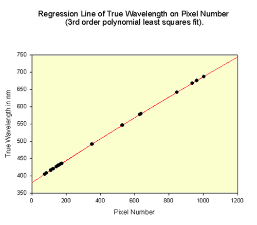
A regression analysis is then performed on the above data with the following result in Figure 1:
Fig. 1 Regression Line Produced from the Calibration Procedure
Evaluating the intercept and the three coefficients determine the relationship between actual wavelength and pixel number. The goodness of fit of the model should be very high, and the correlation coefficient (r2) should be a number very close to 1 (it is 0.9999997 in this example). An F test from an analysis of variance (ANOVA) should similarly produce a large number indicating a high degree of statistical significance. If r2 is not close to 1, this usually indicates that a wavelength value has been mistyped or incorrectly assigned during the procedure.
From the regression analysis, the relationship between the true wavelength and the pixel number in the measured spectra is given by the following expression:
This equation only applies for a given grating and micrometer setting used in the experiment. Should these parameters change a new calibration procedure has to be performed. The calibration parameters (I, C1, C2, C3) are usually stored in a configuration file by the software that is unique to the grating and λ range used. Therefore once a calibration has been carried it does not need to be repeated (unless gratings are changed and/or the detector is moved as mentioned earlier).
Although at first glance it may look straight, the regression line above actually exhibits some slight curvature. A second order quadratic model may have been enough to fit the experimental data, but a 3rd order polynomial takes into account any sigmoidal variation in the data.
In general the dispersion of a grating is not exactly linear in wavelength and deviations from linearity can be both in a positive sense and a negative sense, leading to a very slight s-shaped form of the regression line. The extent of non-linear dispersion in gratings is primarily determined by the accuracy of the ruling engine used to physically rule the grooves on the grating during its manufacture. It is also limited by the machining tolerances of the micrometer wavelength drive in the spectrometer.
Small spectrographs such as the MS125 that employ micrometers to change the wavelength range usually use a sine-bar drive. This is a device built onto the support that holds the grating in the spectrometer. It usually consists of a bar with a hardened steel ball at the end which is in intimate contact with the polished flat end of the micrometer shaft. Small variations in the machining or alignment of the sine-bar drive will also contribute to the small deviations from linearity that are seen in the calibration curve.